14.3. GTApprox Tests
Sections
14.3.1. Methodology
GTApprox is tested by comparing the current version with previous versions in terms of training time and accuracy of the models trained in a number of predefined test cases.
This section provides general test formulation and defines measures. Test case definitions are found in the Test Cases section.
14.3.1.1. Test Case Formulation
For each test case, a multi-dimensional training sample \(\{\mathbf x_n, y_n\}_{n=1}^N\subset {\mathbb R}^{d+1}\) is generated by sampling a scalar-valued response function \(y=f(\mathbf x)\) with \(\mathbf x\in{\mathbb R}^d\). This sample is used to construct the approximation \(\widehat{f}\) of the response function \(f\). Then, the predictive accuracy of the approximation is measured using an independent test sample \(\{\mathbf x'_k, y'_k\}_{k=1}^K\subset {\mathbb R}^{d+1}\) generated by sampling the same response function \(f\) (see Accuracy Measures).
Therefore, a test case is defined by:
- The response function \(f\). To make test cases easily portable and reproducible, most response functions used in testing are defined by analytical formulas.
- The design space \(\mathcal D\) on which the response function is considered. Typically this is the unit hypercube \([0,1]^d\).
- The design of the experiment used to generate a training sample in \(\mathcal D\), which may be one of the following:
- “rnd”: random sample
- “unif”: uniform grid
- “cornrnd”: random sample with additional points in the corners of the design space
- “lhc”: Latin hypercube
- The size \(N\) of a training sample.
Regardless of the size and type of a training sample, a large random subset of the design space is used as a test sample, in order to increase the statistical reliability of error estimates.
14.3.1.2. Test Naming Rules
Each test case has a name in the form of prefix-function-doe, where:
- prefix is the name of function set (for internal use),
- function is the name of the function as these names are listed in the Test Cases section, and
- doe is the technique used to generate a training sample (“rnd”, “unif”, “cornrnd” or “lhc”, see above).
Sample size is not included in the name, since each test is conducted for a variety of the training sample sizes, which are listed in the spreadsheets found in the GTApprox Test Report.
14.3.1.3. Accuracy Measures
After an approximation \(\widehat{f}\) has been constructed for a particular test case, its accuracy is evaluated on a test sample \(\{\mathbf x'_k, y'_k=f(\mathbf x'_k)\}_{k=1}^K\). Let \(\Delta_k\) denote the difference between the value predicted by the approximation at the \(k\)-th point and the respective true value of the response function:
Then, common accuracy measures are:
Mean absolute error (MAE):
\[\mathrm{MAE } = \frac{1}{K}\sum_{k=1}^K|\Delta_k|\]Root-mean-square error (RMS):
\[\mathrm{RMS } = \sqrt{\frac{\sum_{k=1}^K\Delta_k^2}{K}}\]Maximum error (MAX):
\[\mathrm{MAX } = \max_{k=1,\dots,K}|\Delta_k|\]Relative root-mean-square error (RRMS):
\[\mathrm{RRMS } = \sqrt{\frac{\sum_{k=1}^K\Delta_k^2}{\sum_{k=1}^K\widetilde{\Delta}_k^2}} ,\]where \(\widetilde{\Delta}_k\) is the difference between the response function and its mean value estimated on the test set:
\[\widetilde{\Delta}_k = f(\mathbf x_k')-\frac{1}{K}\sum_{s=1}^K f(\mathbf x'_s).\]
14.3.1.4. Performance Profile
The performance profile is a function showing the share of test cases where the relative error is below the given value \(a\). Let \(\mathcal A\) be an approximation tool (algorithm). Then, after constructing approximations in several test cases using \(\mathcal A\) and evaluating their accuracy, one can plot the performance profile \(P_{\mathcal A}\):
where \({Perf}_{\mathcal A}({\rm TC})\) is the performance characteristic, which may be either of:
- RRMS error of the approximation obtained with the algorithm \(\mathcal A\) in test case \(TC\) (in this case, \(P_{\mathcal A}(1)\) is the share of test cases where the algorithm \(\mathcal A\) has advantage over the trivial prediction of the response function by its mean value).
- Time taken to construct the approximation with the algorithm \(\mathcal A\) in test case \(TC\).
The performance profile function \(P_{\mathcal A}\) monotonically increases from 0 to 1; better algorithms (with regard to the selected performance characteristic \({Perf}_{\mathcal A}\)) correspond to higher-lying performance profiles.
14.3.2. Test Cases
This section describes individual GTApprox test cases (actual test settings).
Each case is defined by a response function (listed in sections below), design space \(\mathcal D\), a design of the experiment and training sample size.
For all tests, \(\mathcal D = [0,1]^d\) if not stated otherwise.
Each response function is tested with the four DoE generation techniques described in Test Case Formulation.
Each test is conducted for a variety of the training sample sizes, which are listed in the spreadsheets found in the GTApprox Test Report. The test sample is always a large random subset of the design space.
Note
Following sections denote \(\mathbf x=(x_1,\ldots,x_d)\).
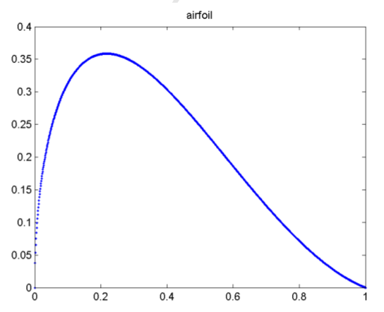
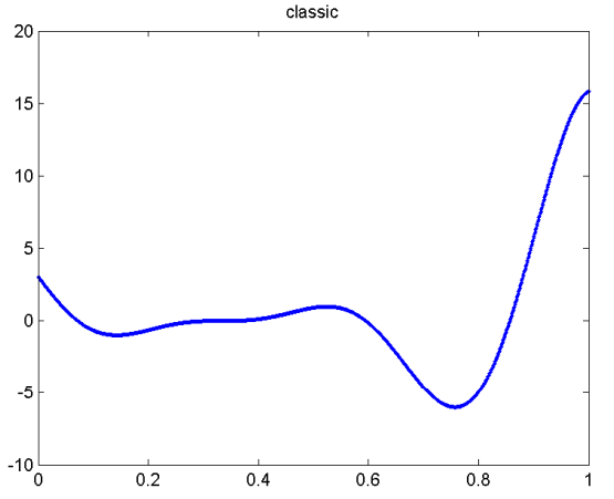
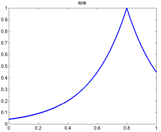
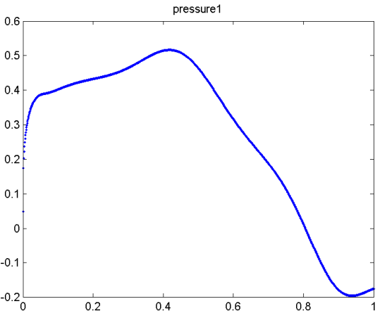
14.3.2.1. 1-Dimensional
airfoil
classic
kink
pressure1
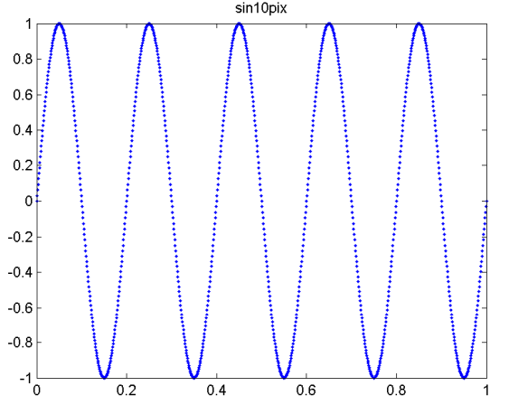
sin10pix
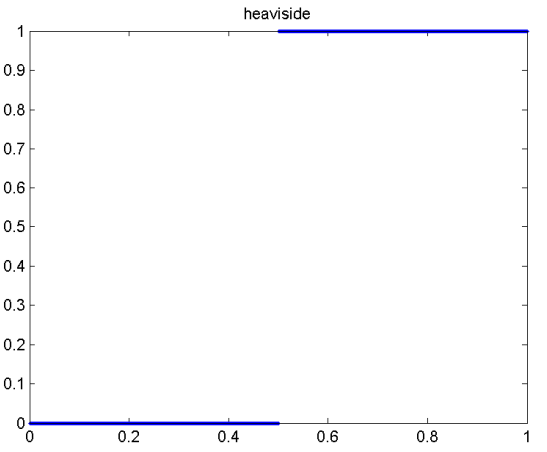
heaviside
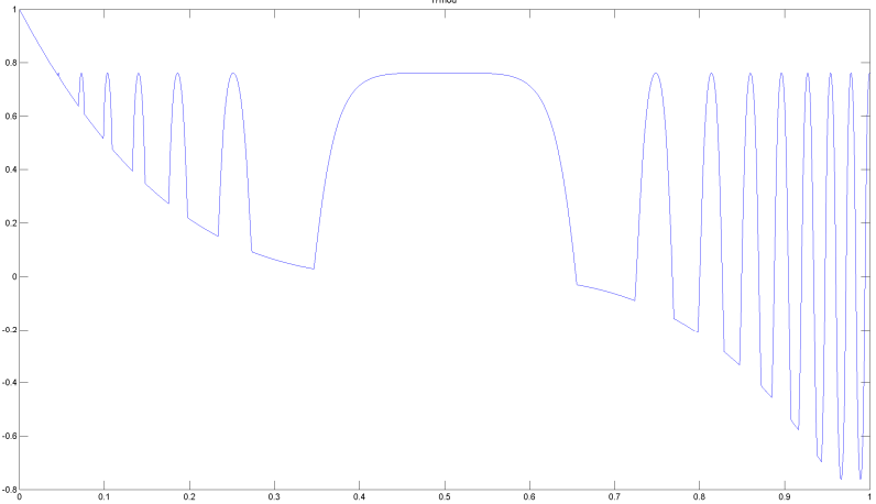
f7mod
14.3.2.2. 2-Dimensional
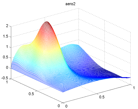
aero2
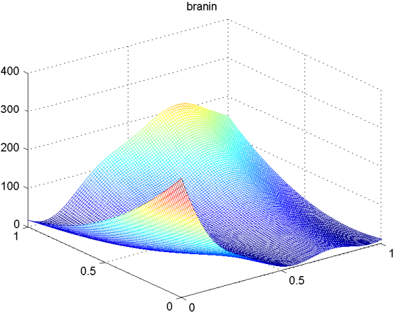
branin
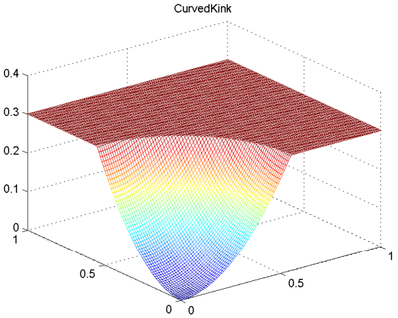
CurvedKink
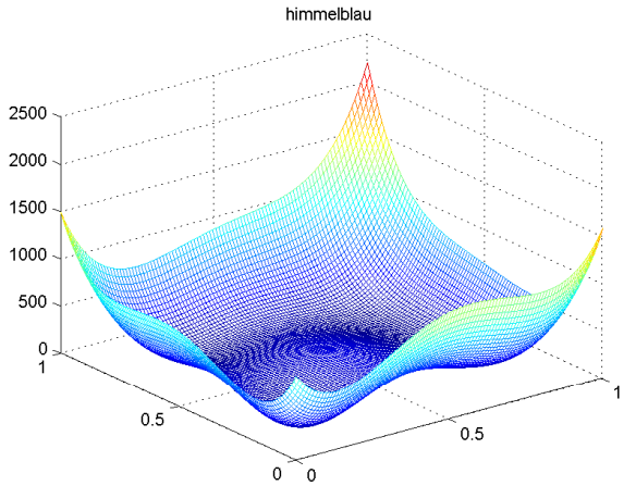
himmelblau
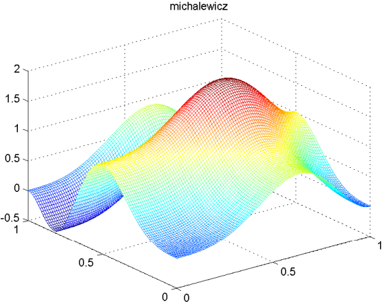
michalewicz
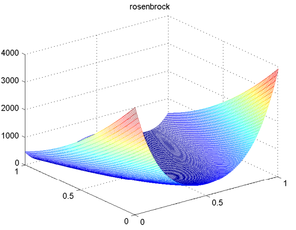
rosenbrock
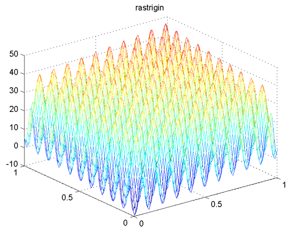
rastrigin
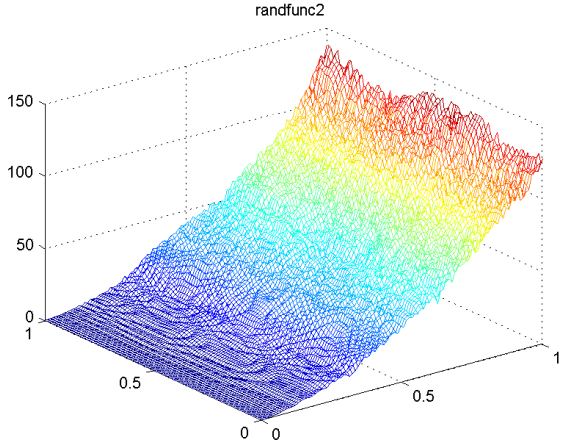
randfunc2
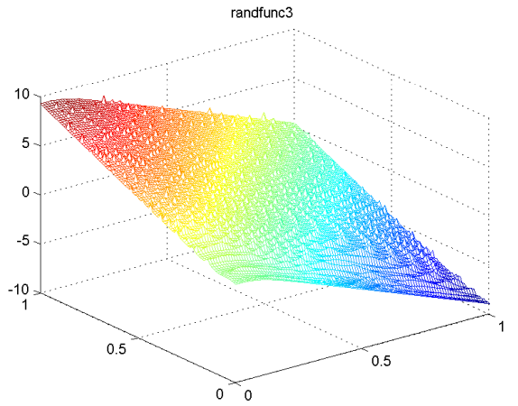
randfunc3
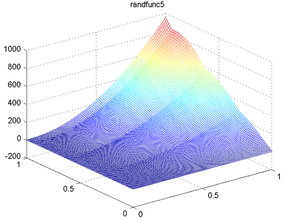
randfunc5
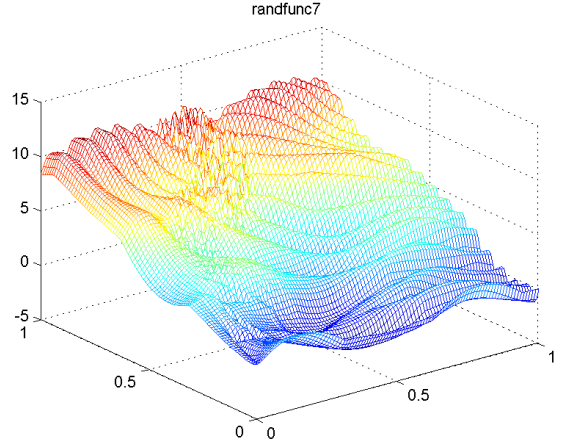
randfunc7
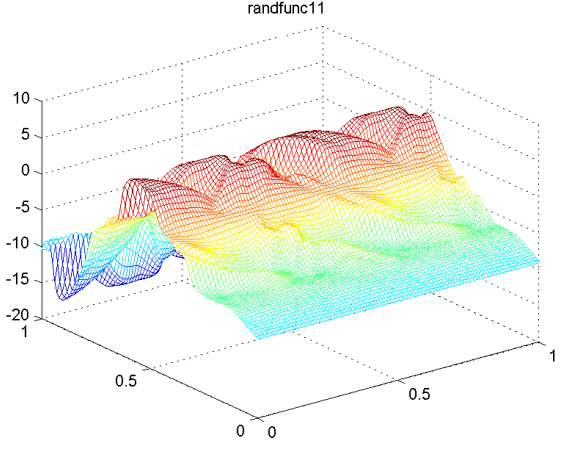
randfunc11
14.3.2.3. 3-Dimensional
The following functions are sampled on the design space \([-1,1]^d\) with various values of \(d\).
linear
sinusoid
ellipsoidal
ackley
whitley