3.5. Numerical Methods

This page lists notable numerical methods used or implemented in GTOpt.

3.5.1. General

Very brief sketch of utilized and implemented numerical methods, not directly related to optimization per se follows.

1. Linear algebra.

   We use functionality provided by the Eigen template library. However, there are notable functionality missing in Eigen library, which had been developed in-house:

   • Block indefinite LDLT factorization and related things.
   • Eigen system updates with respect to rank-1 modifications.
   • Specialized solver of KKT (saddle-point) linear systems, including:
     • Adaptive selection of block indefinite factorization and iterative algorithms.
     • Automatic inertia controlling.
   • Large scale and special linear systems solvers with:
     • Automatic selection of iterative (LSMR, MINRES, PCG) and direct methods.
     • Highly sophisticated iterative preconditioners (SAINV, RIC).
   • Many other less notable routines.

2. Line search methods.

   Variety of inexact methods (Armijo, Goldstein, Wolfe), modified to respect our requirements (data noisiness, occasional undefined model behavior and such).

3. Efficient methods of Pareto-optimal subset selection.

4. A lot of other routines which were easier to implement in-house than to adapt freely available implementations.

3.5.2. Multi-Objective Descent

This is a special-purpose family of algorithms, used almost everywhere within the GTOpt stack. Their ultimate aim is to provide an universal optimality estimation of current iterate \(x_k\), suitable for single- and multi-objective problems, with or without constraints. Simultaneously, the direction of steepest or Quasi-Newton descent is to be provided (it generalizes the notion of steepest and QN descent in familiar single-objective unconstrained case).

3.5.2.1. Optimal Descent

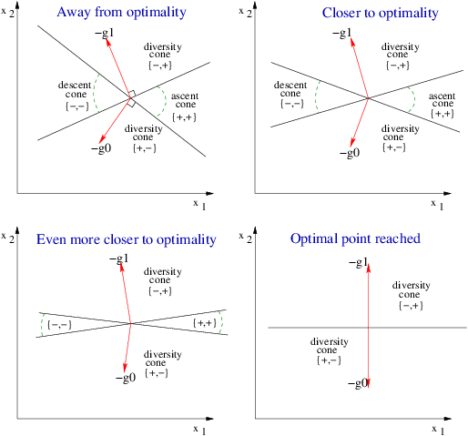
Mathematically, we would like to find (or ensure the absence of) a direction \(d\) such that:

• \(d\) is descent direction for all objectives:

  \[d\cdot \nabla \, f^i ~\le~ 0 \qquad \forall i\]

• \(d\) violates none of imposed bounds in linear approximation

  \[ \begin{align}\begin{aligned}c^j_L \,\le\, c^j ~+~ d\cdot \nabla \,c^j \,\le\, c^j_U \qquad \forall j\\x^k_L \,\le\, x^k ~+~ d \,\le\, x^k_U \qquad \forall k\end{aligned}\end{align} \]

Generically, there is a whole variety of solutions (descent cone). Which one is the most appropriate?

Issue is not related to the constraints, so let’s consider the case \(M=0\) for a while. Normally, for \(K=1\) we take direction of maximal decrease. For \(K>1\) we similar would like to maximally reduce all objectives:

\[\begin{split}\min\limits_{d} \max\limits_i \, d\cdot \nabla \, f^i \quad \Leftrightarrow \quad \begin{array}{cc} \min\limits_{d,t} & t \\ \mbox{s.t.} & d\cdot \nabla \, f^i \,\le\, t \end{array}\end{split}\]

supplemented with the requirement \(|d|_\infty \le 1\) (or anything similar to kill dangerous freedom \(d \to \alpha d\)). Therefore we are invited to solve linear optimization problem to determine optimal descent:

\[\begin{split}\begin{array}{c} \min\limits_{d,t} \, t \\ d\cdot \nabla \, f^i \le t \\ s^j \,\, d\cdot \nabla \, c^j \le t \quad j \in {\cal A} \\ \end{array}\qquad \forall k \,: \,\,d_k \in \left\{ \begin{array}{cc} ~[0:1] & x_k \,\,\,\mbox{is lower-active} \\ ~[-1:0] & x_k \,\,\, \mbox{is upper-active} \\ ~[-1:1] & \,\,\, \mbox{otherwise} \\ \end{array} \right.\end{split}\]

Comments:

• \(t\) directly provides the optimality measure of current iterate.
• \(t\) in constraints-related inequalities serves as regulator, away from optimality it additionally bends descent \(d\) towards the feasible domain.
• Active box bounds had been traded for modified box bounds on \(d\).

3.5.2.2. Quasi-Newton Descent

Similar to well-known single-objective case, constructed steepest descent direction is not perfect:

• Reveals slow convergence if used in iterative line-search based algorithms.
• Badly scaled search direction \(d\): give essentially no predictions on what is the optimal step size.

Remedy is to include second approximations. Basic equations become:

\[\begin{split}\min\limits_{d} \max\limits_i \, [ d\cdot \nabla \, f^i + 1/2 \, d H^i d ] \quad \Leftrightarrow \quad \begin{array}{c} \min\limits_{d,t} \,\, t \\ d\cdot \nabla \, f^i + 1/2 \, d H^i d \,\le\, t \end{array}\end{split}\]

Notes:

• There are no reasons to require \(H^i > 0 ~ \forall i\).
• Hard to solve, but internal and hence cheap by definition (but we must have a mean to solve it).

Generalization to the case of constrained multi-objective problems is trivial and is not presented.