12.5. GTDF¶

Examples

GTDF vs GTApprox

12.5.1. GTDF vs GTApprox ¶

This example will illustrate differences in approximations constructed using GTApprox GP, GTDF VFGP, and GTDF VFGP_BB techniques and show how applying GTDF techniques can improve approximation quality provided that an additional low fidelity data sample is available.

The target function we will be trying to approximate is:

\[f_h(x) = (6 x - 2)^2 \sin(12 x - 4)\]

For the example purposes, this function is considered unknown. Its definition appears in the code (see highFidelityFunction()), but we will only use it in generating \(f_h(x)\) values for the high fidelity data sample and for plotting, so the analytical form of the target function is not available to GTApprox or GTDF.

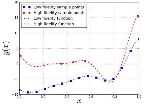
We consider the high fidelity sample to include \(f_h(x)\) values at points \(\mathbf{X}_h = \{0.01, 0.4, 0.45, 0.55, 0.99\}\). The \(\mathbf{X}_h\) list will be the input of highFidelityFunction() which will generate \(f_h(x)\) values for the high fidelity sample.

To generate the low fidelity sample, we will need an additional function lowFidelityFunction(). Its analytical form is:

\[f_l(x) = 0.5 f_h(x) + 10 (x - 0.5) - 5\]

The lowFidelityFunction() definition will be used in sample generation and plotting, but also later we will introduce a blackbox to be used by GTDF VFGP_BB technique which evaluates this function at the given point. Again, this does not mean that analytical form of this function is available to GTApprox or GTDF: GTDF can only request function values from the blackbox, not the function itself.

We consider the low fidelity sample to include \(f_l(x)\) values at points \(\mathbf{X}_l = \{0, 0.1, 0.2, 0.3, 0.4, 0.5, 0.6, 0.7, 0.8, 0.9, 1\}\) - this list will be the input of lowFidelityFunction() which will generate \(f_l(x)\) values for the low fidelity sample.

Following figure shows \(f_h(x)\) and \(f_l(x)\) plots and sample points distribution:

High and low fidelity sample generating functions.

After generating samples, we construct an approximation model for each technique. GP approximation has no means to properly incorporate the data provided by the low fidelity sample into the model building process, so GTApprox GP will only use the high fidelity sample. GTDF VFGP input is both high and low fidelity samples, and approximation quality is better compared to the GP model. GTDF VFGP_BB uses the high fidelity sample and may request additional points from the blackbox containing the low fidelity function, and this further improves the approximation model.

Start with importing modules. Note that this example requires Matplotlib for plotting; it is recommended to use at least version 1.1 to render the plots correctly. We also use a fixed random seed to make the results reproducible:

from da.p7core import gtapprox
from da.p7core import gtdf
from da.p7core import blackbox
from da.p7core import loggers

import numpy as np
import matplotlib.pyplot as plt

import os

Define the \(f_h(x)\) and \(f_l(x)\) functions:

# functions to approximate
def highFidelityFunction(x):
  return (6. * x - 2.) ** 2. * np.sin(12. * x - 4.)

def lowFidelityFunction(x):
  return 0.5 * highFidelityFunction(x) + 10. * (x - 0.5) - 5.

Training samples generation method:

def getTrainData():
  '''
  Generate training samples.
  '''
  lowFidelityPoints = np.linspace(0., 1., 15)
  highFidelityPoints = np.array([0.01, 0.35, 0.45, 0.55, 0.99])

  lowFidelityValues = lowFidelityFunction(lowFidelityPoints)
  highFidelityValues = highFidelityFunction(highFidelityPoints)

  return lowFidelityPoints, lowFidelityValues, highFidelityPoints, highFidelityValues

Now we can define methods to build GTApprox GP and GTDF VFGP models. GP technique uses the high fidelity sample only:

def trainGpModel(highFidelityTrainPoints, highFidelityTrainValues):
  '''
  Build GTApprox model using GP technique.
  '''
  # create builder
  builder = gtapprox.Builder()
  # set logger
  logger = loggers.StreamLogger()
  builder.set_logger(logger)
  # setup options
  options = {
  'GTApprox/Technique': 'GP',
  'GTApprox/LogLevel': 'Info',
  }
  builder.options.set(options)
  # train GT Approx model
  return builder.build(highFidelityTrainPoints, highFidelityTrainValues)

VFGP technique uses both samples:

def trainVfgpModel(highFidelityTrainPoints, highFidelityTrainValues, lowFidelityTrainPoints, lowFidelityTrainValues):
  '''
  Build GTDF model using VFGP technique.
  '''
  # create builder
  builder = gtdf.Builder()
  # set logger
  logger = loggers.StreamLogger()
  builder.set_logger(logger)
  # setup options
  options = {
  'GTDF/Technique': 'VFGP',
  'GTDF/LogLevel': 'Info',
  }
  builder.options.set(options)
  # train GT DF model
  return builder.build(highFidelityTrainPoints, highFidelityTrainValues, lowFidelityTrainPoints, lowFidelityTrainValues)

To use the VFGP_BB technique, we will have to create the blackbox class which will evaluate the low fidelity function at the points requested by GTDF builder. In real world case, the evaluate() method of this class will typically contain a call to some external function which returns the values needed.

class LowFidelityFunctionBlackBox(blackbox.Blackbox):
  '''
  Blackbox class for evaluating low fidelity function.
  '''
  def __init__(self):
    blackbox.Blackbox.__init__(self)

  def prepare_blackbox(self):
    self.add_variable((0, 1))
    self.add_response()

  # low fidelity function evaluation
  def evaluate(self, points):
    result = []
    for point in points:
      result.append([lowFidelityFunction(point[0])])
    return result

Now we can build the GTDF_BB model. This method accepts the high fidelity sample and an instance of LowFidelityFunctionBlackBox class as a parameter lowFidelityFunctionBlackBox:

def trainVfgpBbModel(highFidelityTrainPoints, highFidelityTrainValues, lowFidelityFunctionBlackBox):
  '''
  Build GTDF model using VFGP_BB technique.
  '''
  # create builder
  builder = gtdf.Builder()
  # set logger
  logger = loggers.StreamLogger()
  builder.set_logger(logger)
  # setup options
  options = {
  'GTDF/Technique': 'VFGP_BB',
  'GTDF/LogLevel': 'Info',
  }
  builder.options.set(options)
  # train blackbox-df model
  return builder.build_BB(highFidelityTrainPoints, highFidelityTrainValues, lowFidelityFunctionBlackBox)

Next is the method to build the three models using the generated samples. For GTDF_BB, we also create an instance of LowFidelityFunctionBlackBox class inside this method and pass it to trainVfgpBbModel():

def buildModels(lowFidelityTrainPoints, lowFidelityTrainValues, highFidelityTrainPoints, highFidelityTrainValues):
  '''
  Build surrogate models.
  Three techniques are used to build an approximation: GTApprox GP, GTDF VFGP, GTDF BB VFGP.
  '''
  gtaModel = trainGpModel(highFidelityTrainPoints, highFidelityTrainValues)

  vfgpModel = trainVfgpModel(highFidelityTrainPoints,
                             highFidelityTrainValues,
                             lowFidelityTrainPoints,
                             lowFidelityTrainValues)

  lfBlackBox = LowFidelityFunctionBlackBox()
  blackboxModel = trainVfgpBbModel(highFidelityTrainPoints,
                                   highFidelityTrainValues,
                                   lfBlackBox)

  return gtaModel, vfgpModel, blackboxModel

Following methods will be needed to test models built by buildModels() method:

def getTestData(sampleSize):
  '''
  Generate test data.
  '''
  points = np.reshape(np.linspace(0., 1., sampleSize), (sampleSize, 1))

  lowFidelityValues = lowFidelityFunction(points)
  highFidelityValues = highFidelityFunction(points)

  return points, lowFidelityValues, highFidelityValues

def calculateValues(testPoints, gtaModel, vfgpModel, blackboxModel):
  '''
  Calculate models on given sample.
  '''
  gtaValues = gtaModel.calc(testPoints)
  vfgpValues = vfgpModel.calc(testPoints)
  bbValues = blackboxModel.calc_bb(LowFidelityFunctionBlackBox(), testPoints.tolist())
  return gtaValues, vfgpValues, bbValues

Plotting methods (use Matplotlib and require at least version 1.1 to work correctly):

def plot_train(lowFidelityTrainPoints, lowFidelityTrainValues, highFidelityTrainPoints, highFidelityTrainValues):
  '''
  Visualize training sample.
  '''
  plt.plot(lowFidelityTrainPoints, lowFidelityTrainValues, 'sb', markersize = 7.0, linewidth = 2.0, label = 'Low fidelity sample points')
  plt.plot(highFidelityTrainPoints, highFidelityTrainValues, 'or', markersize = 7.0, linewidth = 2.0, label = 'High fidelity sample points')

def plot_test(testPoints, lowFidelityTestValues, highFidelityTestValues):
  '''
  Visualize test sample.
  '''
  plt.plot(testPoints, lowFidelityTestValues, '-.b', linewidth = 2.0, label = 'Low fidelity function')
  plt.plot(testPoints, highFidelityTestValues, 'r', linestyle = '--', linewidth = 2.0, label = 'High fidelity function')

def plot_approximations(testPoints, gtaValues, vfgpValues, bbValues):
  '''
  Visualize approximations.
  '''
  plt.plot(testPoints, gtaValues, ':m', linewidth = 2.0, label = 'GTApprox GP')
  plt.plot(testPoints, vfgpValues, 'c', linewidth = 2.0, label = 'GTDF VFGP')
  plt.plot(testPoints, bbValues, '--k', linewidth = 2.0, label = 'GTDF BB VFGP')

def show_plots():
  '''
  Configure, show and save plots.
  '''
  plt.xlabel(r'$x$', fontsize = 30)
  plt.ylabel(r'$y(x)$', fontsize = 30)
  plt.grid(True)
  plt.title('GTDF example')
  plt.legend(loc = 'best')
  name = 'gtdf_simple_example'
  plt.savefig(name)
  print('Plot is saved to %s.png' % os.path.join(os.getcwd(), name))
  if 'SUPPRESS_SHOW_PLOTS' not in os.environ:
    plt.show()

In the main workflow, we generate input samples by getTrainData(), pass it to buildModels() to create models, and then calculate model values for the points of the testing sample to obtain plots:

def main():
  """
  Toy example of GTDF usage.
  """
  print('GTDF usage example')
  print('=' * 50)
  print('Generate training sample...')
  trainData = getTrainData()
  print('Build models...')
  models = buildModels(*trainData)
  print('Generate test sample...')
  testPoints, lowFidelityTestValues, highFidelityTestValues = getTestData(1000)
  print('Calculate model values for the test sample...')
  modelsValues = calculateValues(testPoints, *models)
  print('Plotting...')
  figure_handle = plt.figure(figsize=(8.5, 8))
  # visualize training sample
  plot_train(*trainData)
  # visualize test sample
  plot_test(testPoints, lowFidelityTestValues, highFidelityTestValues)
  # visualize approximations
  plot_approximations(testPoints, *modelsValues)
  # show and save plots
  show_plots()

if __name__ == "__main__":
  main()

To run the example, open a command prompt and execute:

python -m da.p7core.examples.gtdf.example_gtdf_simple

You can also get the full code and run the example as a script: example_gtdf_simple.py.

Running the example yields an image with plotted models and high and low fidelity functions:

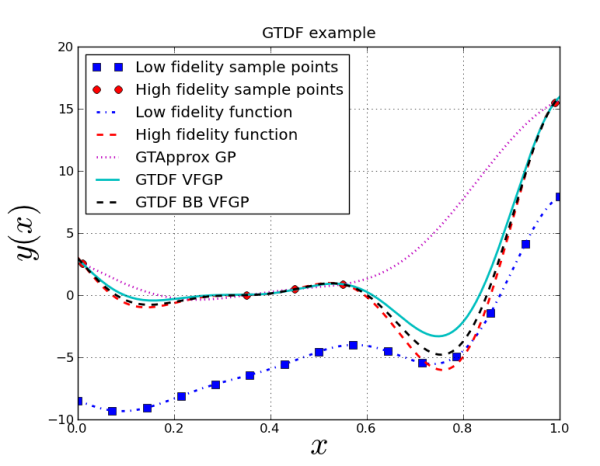
True functions and approximation models.

As you can see, using the low fidelity data increased approximation accuracy (GTDF VFGP curve is closer to the target high fidelity function than GP curve); GTDF VFGP_BB curve is slightly better because this technique can evaluate the low fidelity function at any feasible point and is not limited by the amount of points in the low fidelity sample and their distribution.

More GTDF examples can also be found in Code Samples.

12.5. GTDF¶

12.5.1. GTDF vs GTApprox¶

12.5.1. GTDF vs GTApprox ¶