4.4. Quality Assessment
Sections
4.4.1. Model Validation
Once the model is created, one usually wants to check how accurate it is. To allow this, GTApprox currently supports the following ways to validate the constructed model:
- Accuracy on train set - GTApprox computes model accuracy on training set directly. It is very cheap, so we always do it, but obtained accuracy may be greatly overestimated.
- Internal Validation - optional procedure that validates model on train data by means of cross-validation. IV may significantly increase model building time, but gives reliable accuracy estimates (reliability mostly depends on how good your train sample represents design space).
- Validation on test set - procedure validates the model using given external test sample.
4.4.1.1. Error metrics
In GTApprox we consider a number of error metrics that show various properties of the model. The idea of general model quality can usually be got by looking at this set of computed error metrics.
Let us denote: a training set \(S\) that consists of N=|S| pairs of \(d_{in}\)-dimensional input points \(X\) and \(d_{out}\)-dimensional outputs \(Y\) (\(Y=f(X)\), where \(f\) is some unknown function).
Additionally, the user may provide weights of points in the training set (see Sample Weighting). In other words, each pair \((X_{i}, Y_{i})\) may be additionally related to a weight variable \(W_{i}=W(X_{i}) \geq 0\). For future reference, let’s consider that weights comply with normalization condition:
it means that normalization was applied to initial weights \(W(X_{i}), i=1,\ldots,N\) specified by the user:
Weight variables modify statistical calculations by giving more weight to one type of observations as compared to other ones. When comparing a weighted and unweighted analyses, the key idea is as follows: an unweighted analysis is equivalent to the weighted one when all weights are equal.
We denote considered model as function \(\hat{f}\) that we expect to approximate \(f\) in all design space. Let \(\varepsilon(X) = |\hat{f}(X) - f(X)|\) be the absolute error of prediction in point \(X\).
Let’s sort the set of absolute errors \(\left\{\epsilon(X_{i}),i=1,\ldots,N\right\}\) from smallest to largest. Then, the new ordered sample will be represented by a non-decreasing sequence
where \(\epsilon(X_{(i)})\) stands for the member of the series being at the i-th place to distinguish it from \(\epsilon(X_{i})\).
If weights are specified, the ordered sample will be represented with a sequence of pairs with the first element being arranged in a non-decreasing order:
Note that unweighted ordered sample (1) is equivalent to weighted one (2), if all weights are \(w(X_{(i)})=1/N,i=1,\ldots,N\).
Then construct the empirical cumulative distribution function (ECDF). Recall that the ECDF is a piecewise-constant step function that increases by \(w(X_{(i)})\) for weighted ordered sample (2) and by 1/N for unweighted ordered sample (1) at each data point.
Example.
Let us suppose your data are \(\left\{0.1, 0.19, 0.22, 0.3, 0.37, 0.41, 0.5, 0.61\right\}\). The following graph shows the ECDF for these eight values:
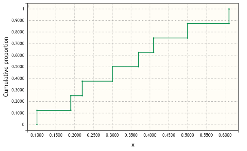
Let the weights for this example be: \(\left\{0.2, 0.05, 0.05, 0.15, 0.25, 0.15, 0.1, 0.05\right\}\). The following graph shows the weighted ECDF for these weights:

The data values are indicated by tick marks along the horizontal axis. To find a quantile, start at some value on the vertical axis, move across until you hit a vertical line, and then drop down to the X axis to find the datum value.
4.4.1.1.1. Componentwise errors
Denote the error on l-th output component at point \(X\) as \(\epsilon\Big(X^{(l)}\Big)\). Then, the ordered sample (1) for l-th output component in case of unweighted sample is
and the ordered sample (2) in case of weighted sample is
Note
Generally, a weight variable can take any non-negative value including 0. If the weight \(w(X)=0\) is specified for a certain point \(X\), such a point is considered insignificant for model quality assessment and may be excluded from the sample (4). For further reference, let’s assume that all points with zero weights have already been excluded, and the ordered sample contain only points with their weights being equal to \(w(X_{(i)})>0, i=1,\ldots,N\).
For each output \(l=1\ldots d_{out}\) GTApprox separately computes the whole set of componentwise error metrics.
- Max — maximum absolute error:
\(Max^{l}\) is the largest order statistic of the ordered sample (3) (or (4)).
Mean - mean absolute error or MAE:
\[{Mean}^{(l)} = \sum_{i=1}^{N}w_{(i)}\epsilon\Big(X_{(i)}^{(l)}\Big)\]
for the weighted ordered sample (4). In case of unweighted sample (3), it can be represented by a well-known formula
\[{Mean}^{(l)} = \frac{1}{N}\sum_{i=1}^{N}\epsilon\Big(X_{(i)}^{(l)}\Big)\]
- Median — median of absolute error:
\({Median}^{(l)}\) is such a value \(\epsilon\Big(X^{(l)}\Big)\) in the ordered sample for which the empirical cumulative distribution function is equal to 0.5.
To find a median with the graph of ECDF, start at the value 0.5 on the vertical axis, move across until you hit a vertical line, and then drop down to the X axis to find the datum value.
- Q0.95 — 95-percent quantile of absolute error:
\(Q0.95^{(l)}\) is such a value \(\epsilon\Big(X^{(l)}\Big)\) in the ordered sample for which the empirical cumulative distribution function is equal to 0.95.
Q0.99 — 99-percent quantile of absolute error:
\(Q0.99^{(l)}\) is such a value \(\epsilon\Big(X^{(l)}\Big)\) in the ordered sample for which the empirical cumulative distribution function is equal to 0.99.
\[{Q0.99}^{(l)} = arg\left\{ECDF(X^{(l)})=0.99\right\}\]
RMS — root-mean-squared error:
\[{RMS}^{(l)} = \sqrt{\sum_{i=1}^{N}w_{(i)}\Big(\epsilon(X_{(i)}^{(l)}})^{2}\Big)\]
for the weighted ordered sample (4). In case of unweighted ordered sample (3), it can be represented by a well-known formula
RRMS — relative root-mean-squared error,
\[{RRMS}^{(l)} = \frac{{RMS}^{(l)}}{\sqrt{var\Big(Y^{(l)} \Big)}}\]where \(var \Big(Y^{(l)} \Big)\) is the variance of \(Y^{(l)}\) on the sample \(S\).
R^2 — coefficient of determination,
\[R^{2(l)}=1.0-\frac{\Big(RMS^{(l)} \Big)^{2}}{var \Big(Y^{(l)} \Big)}\]where \(var \Big(Y^{(l)} \Big)\) is the variance of \(Y^{(l)}\) on the sample \(S\).
4.4.1.1.2. Aggregated errors
In addition to Componentwise errors GTApprox also computes errors aggregated over all outputs.
Max - maximum componentwise error:
\[Max \,err = max \Big( err^{(l)} \Big),\]where \(err^{(l)}\) is considered type of Componentwise errors (for example \(err\) = RRMS).
RMS - root-mean-squared of componentwise errors:
\[RMS \,err = \Big(\frac{1}{d_{out}}\sum_{l=1}^{d_{out}} \Big(err^{(l)}\Big)^2\Big)^{1/2},\]Mean - mean componentwise error:
\[Mean \,err = \frac{1}{d_{out}}\sum_{l=1}^{d_{out}} err^{(l)},\]For aggregated errors numbers we use notation like ‘Mean RRMS’, which means average RRMS value over all output components.
4.4.1.2. Accuracy on train set
After training a model, GTApprox validates it against the training dataset,
calculating various error metrics (see Error metrics),
which are then available from gtapprox.Model.details.
Please note, that accuracy on training set computed in such direct way is almost always significantly underestimates model errors on new data. However if accuracy on training set is poor one should take this as strong signal, that constructed model is to simple to handle provided data. In such case one should consider trying more complex model.
4.4.1.3. Internal Validation
The Internal Validation (IV) procedure is a part of GTApprox providing an estimate of the expected overall accuracy of the approximation algorithm. This estimate is obtained by doing cross-validation (see Cross-validation procedure details) of the algorithm on the training data.
Internal Validation can be enabled or disabled by the GTApprox/InternalValidation option (default is disabled).
The procedure returns a standard set of Error metrics. The result of this procedure can be accessed from the iv_info attribute of the GTApprox Model object.
Details of procedure implementation are provided below.
4.4.1.3.1. Cross-validation procedure details
Cross-validation is a well-established way of statistical assessment of the algorithm’s efficiency on the given training set (see, e.g. [Arlot2010], [Geisser1993]). It should be stressed, however, that it does not directly estimate the predictive power of the model \(\hat{f}\). Rather, the purpose of cross-validation is to assess the efficiency of the approximation algorithm \(A\) (with corresponding parameters specified) on various subsets of the available data, assuming that the conclusions can be extended to the (unavailable) observations from the total design space and final model constructed on all the data.
The procedure depends on the following parameters that can be set by using GTApprox options:
- \(N_{ss}\) — number of subsets that the original training set \(S\) is divided into, where \(2 \leq N_{ss} \leq |S|\). This number is determined by the options GTApprox/IVSubsetCount and GTApprox/IVSubsetSize.
- \(N_{tr}\) — number of validation sessions, where \(N_{tr} \geq 1\). This number is determined by the GTApprox/IVTrainingCount option, which sets an upper limit for \(N_{tr}\), and the number of subsets \(N_{ss}\). The applied value of \(N_{tr}\) is the minimum of GTApprox/IVTrainingCount and \(N_{ss}\).
- The seed for the pseudo-random division of \(S\) into subsets. This seed is set by the option GTApprox/IVSeed.
The default \(N_{ss}\) value is selected automatically depending on the training set size \(|S|\), and is applied when both the GTApprox/IVSubsetCount and GTApprox/IVSubsetSize options are default.
To set the number of training subsets \(N_{ss}\) to a specific value, use the GTApprox/IVSubsetCount option. In this case, GTApprox/IVSubsetSize must be kept default. The training set \(S\) is divided into approximately equal in size subsets, the number of which is equal to the value of the GTApprox/IVSubsetCount option.
To set the size of the training subset to a specific value, use the GTApprox/IVSubsetSize option. In this case, GTApprox/IVSubsetCount must be kept default. The training set \(S\) is divided into subsets, each having size as close as possible to the value of the GTApprox/IVSubsetSize option. The value of \(N_{ss}\) is equal to the number of subsets obtained in this way.
The latter option makes it easy to enable leave-one-out cross-validation by setting GTApprox/IVSubsetSize to 1. In this case, \(N_{ss}=|S|\), which yields the leave-one-out cross-validation with \(N_{tr}\) points to leave out (note that \(N_{tr}\) may be less than \(N_{ss}\)). The full leave-one-out cross-validation requires that \(N_{tr} \geq N_{ss}=|S|\), and can be achieved by setting GTApprox/IVTrainingCount to a sufficiently large value, in order to meet the required condition.
The cross-validation procedure used in GTApprox includes the following steps:
From the options’ values and the properties of the training set \(S\), GTApprox determines the appropriate model training algorithm \(A\).
The algorithm \(A\) is used to obtain the main approximation \(\hat{f}\), which is the final model provided to the user.
Changed in version 6.14: cross validation starts only after the main model is trained. In previous versions, cross validation was performed before training the main model.
Note
Cross validation is also used internally by the smart training procedure (see Smart Training), but only in the case when there is no test sample to estimate quality of intermediate models. In this case, the full training set \(S\) is used only to train the final model with optimal training settings, so step 2 is essentially skipped for intermediate models.
After that, GTApprox starts cross validation of the algorithm \(A\) on the sample \(S\).
- The set \(S\) is randomly divided into \(N_{ss}\) disjoint subsets \((S_k)^{N_{ss}}_{k=1}\) of approximately equal size.
- For each \(k=1,\ldots,N_{tr}\), an \(A\)-based approximation \(\hat{f_k}\) is trained on the subset \(S\setminus S_k\), and its errors \(E_{k,l}\) of one of the three standard types, MAE, RMS and RRMS (see Error metrics) are computed on the complementary test subset \(S_k\), separately for each scalar component \(l=1,\ldots,d_{out}\) of the output.
- The cross-validation errors \((E^{cv}_l)_{l=1}^{d_{out}}\) are computed as the median values of the errors \(E_{k, l}\) over the training/validation iterations \(k=1,\ldots,N_{tr}\).
- The total cross-validation Componentwise errors and Aggregated errors are computed.
The parametrization of the IV procedure by \(N_{ss}\) and \(N_{tr}\) endows it with additional flexibility while also allowing common types of validation:
- Standard full leave-one-out cross-validation is achieved by either of:
- setting \(N_{tr}=N_{ss}=|S|\), or
- setting GTApprox/IVSubsetSize to
1and GTApprox/IVTrainingCount to an arbitrarily high value greater than \(|S|\), in which case GTApprox sets \(N_{tr}=N_{ss}=|S|\) automatically.
- \(N_{tr}=1\) corresponds to a single instance of training and validation, where the initial set \(S\) is divided into the training and test subsets \(S_{train}\), \(S_{test}\) so that \(\frac{|S_{test}|}{|S|}\approx\frac{1}{N_{ss}}\) and \(\frac{|S_{train}|}{|S|}\approx\frac{N_{ss}-1}{N_{ss}}\).
Note, however, that, regardless of the settings of the IV procedure, its efficiency for any conclusions related to points outside the training sample, or to the total design space, is fundamentally restricted by the total amount of information contained in the training set and the actual validity of the inference assumptions.
Note
Since only a subset of the training sample is used for approximation construction during Internal Validation, enabling GTApprox/InternalValidation changes the required minimum sample size \(|S|\) (see Sample Size Requirements).
Note
GTApprox provides a way to save outputs calculated during IV procedure in each point, which may be useful if you want to compute your own error metrics or plot the error distribution. To save outputs of models \(\hat{f_k}\) trained during cross-validation, enable the GTApprox/IVSavePredictions option (default is disabled).
It should be stressed that though cross-validation is a conventional way to assess the efficiency of the approximating method on the given data, a precise estimate of the errors on the whole design space can only be obtained by validating the approximation \(\hat{f}\) against a holdout test sample, which is sufficiently large and properly selected.
However, if the user already has a test sample, applying the approximation to it and computing the desired accuracy characteristics are straightforward operations, and the user should have no difficulty in performing them, see below.
4.4.1.4. Validation on test set
GTApprox allows to estimate model accuracy on a given test sample.
To do it user should call validate() method of GTApprox Model() object.
Method computes predictions for given test inputs and compares them with given test outputs, by computing standard set of Error metrics.
Note
If the points in the test set are too close to the points from the training set, model may still underestimate prediction errors.
4.4.2. Evaluation of accuracy in given point
Accuracy Evaluation (AE) is a part of GTApprox whose purpose is to estimate the accuracy of the constructed approximation at given points of the design space. If AE is turned on, then the constructed model contains, in addition to the approximation \(\hat{f}:R^{d_{in}}\to R^{d_{out}}\), the AE prediction \(\sigma:R^{d_{in}}\to R_+^{d_{out}}\) and the gradient of AE \(\nabla \sigma:R^{d_{in}}\to R^{d_{in} \times d_{out}}\).
AE is turned on or off by the option GTApprox/AccuracyEvaluation (default value is off).
AE prediction is performed separately for each of the \(d_{out}\) scalar outputs of the response. In the following, it is assumed for simplicity of the exposition and without loss of generality that the response has a single scalar component (\(d_{out}=1\)).
The value \(\sigma(X)\) characterizes the expected value of the approximation error \(|\hat{f}(X)-f(X)|\) at the point \(X\). A typical example of AE prediction is shown in Figure below. An approximation b) is constructed using a training set with DoE shown in a). The AE prediction is shown in d); also, its level sets are shown in c). We see that, on the whole, AE predicts larger error at the points further away from the training DoE. Also, the predicted error is usually larger at the boundaries of the design space. See Section Example.
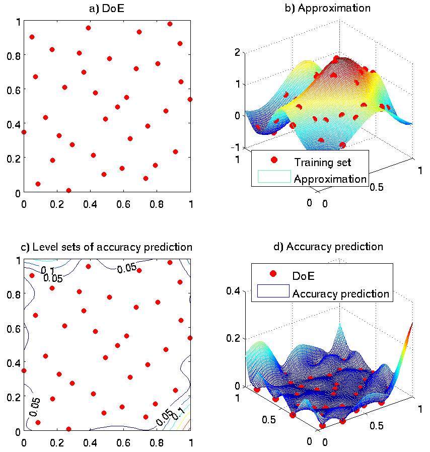
Figure: An example of accuracy prediction in GTApprox.
Note
This image was obtained using an older pSeven Core version. Actual results in the current version may differ.
The following notes explain the functionality of AE in more detail.
The AE prediction is only an “educated guess” of approximation’s error. It is not possible, in general, to predict the exact values of the error. AE predictions should by no means be considered as a guarantee that the actual error is restricted to certain limits.
The AE prediction is usually more efficient in terms of the correlation with the actual approximation errors rather than \(matching\) these errors. In other words, AE predictions are more relevant for estimating relative magnitude of error at different points of the design space. See examples further in this chapter.
In general, the AE prediction \(\sigma\) reflects both of the two sources of the error:
- uncertainty of prediction;
- discrepancy between the approximation \(\hat{f}\) and the training data, resulting from smoothing and a lack of interpolation.
The latter factor is present only for non-interpolating approximations. * The prediction \(\sigma\) has the following general properties:
- \(\sigma\) is a continuous function;
- if the approximation \(\hat{f}\) is interpolating, then at the training DoE points \(X_k\) holds \(\sigma(X_k)=0\);
AE is available in GTApprox for the following approximation techniques: 1D Splines with tension, Gaussian Processes, High Dimensional Approximation combined with Gaussian Processes, Sparse Gaussian Process (see Section Techniques).
The specific algorithms of error prediction depend on particular approximation techniques:
Gaussian-Process-based techniques (GP, HDAGP, SGP) estimate the error using the standard deviations of the Guassian process at particular points, see [Rasmussen2005] .
For Splines with Tension, the error is estimated by combining two different approaches:
- comparison of the constructed spline with splines of a lower order;
- using as a measure of error the distance to the training DoE, rescaled by an overall factor determined via cross-validation.
The default technique for very large training sets (\(>10000\)) in dimensions \(d_{in}>1\) is High Dimensional Approximation, which means that, by default, AE is not available for such training sets. The user can choose Gaussian Processes or High Dimensional Approximation combined with Gaussian Processes as the approximation technique in such cases, but these techniques have high computer memory requirements, which may render the processing of the very large training set infeasible. In fact, for large training sets the discrepancy \(|\hat{f} - f|\) tends to be a highly oscillating function (see, e.g., the example in Section \(Adaptive DoE example\)), and the resolution and reproduction of these oscillations are computationally expensive. Another option, if AE is required, is to use Sparse Gaussian Process, which is available by default for sample sizes between 1000 and 10000. This technique trains the approximation using only a properly chosen subset of a manageable size in the whole training set.
4.4.2.1. Example
In this section we compare performance of AE in a noisy 1D problem with interpolation turned on or off. We select Gaussian Processes as the approximation technique. Gaussian Processes supports the interpolation mode but is not necessarily interpolating by default, see Section Exact Fit. (Note that the default 1D technique is SPLT which is always interpolating in GTApprox, see Section 1D Splines with tension.)
The training data is noisy, and the DoE is gapped. The result of applying GTApprox with interpolation mode turned on or off is shown in Figure below. Note that the forms of the approximation as well as the error prediction are quite different in these two cases. If the interpolation mode is turned on, then the tool perceives the local oscillations as an essential feature of the data and accurately reproduces the provided values. Accordingly, the predicted error vanishes at the points of the training DoE. In the domain where these points have a higher density, the predicted error is low, but in the DoE’s gaps it is large.
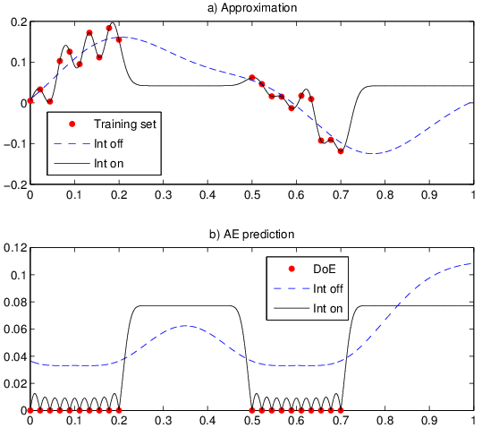
Figure: AE predictions with interpolation on or off.
Note
This image was obtained using an older pSeven Core version. Actual results in the current version may differ.
In contrast, in the default, non-interpolating mode, the tool perceives the local oscillations as a noise and smooths the training data. The perceived uniformly high level of noise makes the tool add a constant to the error prediction, so that it is uniformly bounded away from zero. Another factor which affects the error prediction, the uncertainty growing with the distance to the training DoE, is also present here.