12.6. GTDoE

12.6.1. Monte Carlo Integration

This example performs Monte Carlo integration of multidimensional integral using GTDoE for sample points generation.

The task is (for any fixed \(d\)):

\[\text{Calculate:}\ I_d = \int \ \ldots \ \int _{[0,1]^d} \prod _{k=1}^d k\cos (kx_k) dx_k\]

Correct answer is \(I_d= \prod _{k=1}^d \sin (k)\)

One way to calculate this integral is numerical integration using random sampling (Monte Carlo integration). The result of such integration is highly dependent on the random point generation method. We test available sequential GTDoE techniques and show that sequential techniques with low discrepancy give much better accuracy and faster convergence than plain random sampling.

Begin with importing modules. Note that this example requires SciPy and Matplotlib (for plotting); also, it is recommended to use matplotlib version 1.1 or later for the plots to be displayed correctly.

from da.p7core import gtdoe
from da.p7core.loggers import StreamLogger

import os
import numpy as np
import matplotlib.pyplot as plt

Create a list of techniques to iterate over:

seqTechniqes = {'RandomSeq' : u'Random sampling',
                'SobolSeq' : u'Sobol sequence',
                'FaureSeq' : u'Faure sequence',
                'HaltonSeq' : u'Halton sequence'}

Parametrize the task so we can test the techniques for various dimensions dim. The step parameter is an amount of points added on each Monte Carlo iteration, until the total amount of points used reaches maxPoints:

def monteCarloIncremental(dim, maxPoints, step):

Inside monteCarloIncremental() we begin with printing current task setup and calculating the exact value of integral using the analytical definition of the result \(I_d= \prod _{k=1}^d \sin (k)\):

  print('=' * 50)
  print('Run GTDoE MonteCarlo example with the following inputs: ')
  print('Dimension: %s' % dim)
  print('Number of points: %s' % maxPoints)
  print('Step: %s' % step)
  print('Techniques: %s' % list(seqTechniqes.keys()))
  print('=' * 50)
  print('Calculating exact value of the integral.')
  correctValue  = np.prod([np.sin(i+1) for i in range(dim)])
  print("Correct value: %f" % correctValue)

Next, create a DoE generator for each technique and generate the point sequence. Note we set a fixed random seed and require generation to be deterministic to ensure that results are reproducible:

  techDrivers = {}
  pointGens   = {}
  techY       = {}
  sums        = {}

  print('Create a generator for each DoE technique.')
  bounds = ([0.] *dim, [1.] *dim)
  for tech in seqTechniqes:
    # initialize generator
    techDrivers[tech] = gtdoe.Generator()
    # set options
    techDrivers[tech].options.set('GTDoE/Seed', '100')
    techDrivers[tech].options.set('GTDoE/Deterministic', True)
    techDrivers[tech].options.set('GTDoE/Technique', tech)
    # generate points
    pointGens[tech] = techDrivers[tech].generate(bounds)
    sums[tech] = 0.0
    techY[tech] = []

Perform Monte Carlo integration gradually increasing the number of points and calculating absolute error each time another sample of deltaPoints is added. Error values are stored in techY for each technique; further we will use these values to illustrate convergence on a plot:

  deltaPoints = step
  totalPoints = 0

  print('Perform Monte Carlo integration using different techniques.')
  pointsArray = []
  while totalPoints <= maxPoints:
    print('Points: %d / %d          \r' % (totalPoints, maxPoints))
    for (tech, name) in seqTechniqes.items():
      points = pointGens[tech].take(deltaPoints)
      value = np.sum(np.prod(np.array([(i+1.0) *np.cos((i+1.0)*points[:,i]) for i in range(dim)]).T, axis=1) / deltaPoints)
      sums[tech] = sums[tech] + value
      techY[tech].append(np.abs(sums[tech] / (totalPoints / deltaPoints + 1) - correctValue))
    totalPoints = totalPoints + deltaPoints
    pointsArray.append(totalPoints)

Results output and plotting (plotting uses Matplotlib and requires at least version 1.1 to be displayed correctly):

  # print and visualize results
  plt.figure(0, figsize=(9, 8), dpi=100)

  for tech in sorted(seqTechniqes.keys()):
    print('Technique "%s", result: %f' % (seqTechniqes[tech], sums[tech] / (totalPoints / deltaPoints)))
    coeff = np.polyfit(pointsArray, techY[tech], 1)
    yV = [np.polyval(coeff, x) for x in pointsArray[:-10]]
    plt.semilogy(pointsArray[:-10], yV, label = seqTechniqes[tech])

  # configure plot
  plt.legend(loc = 'best')
  plt.ylabel(u'Error')
  plt.xlabel(u'N')
  plt.title(u'Monte Carlo integration, dimensionality: %d' % dim)
  name = 'doe_montecarlo_' + str(dim)
  plt.savefig(name)
  print('Plot is saved to %s.png' % os.path.join(os.getcwd(), name))
  if 'SUPPRESS_SHOW_PLOTS' not in os.environ:
    print('Close window to continue script.')
    plt.show()

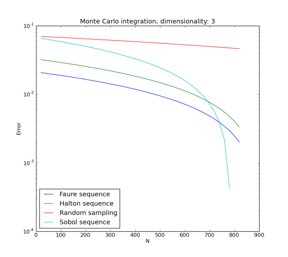
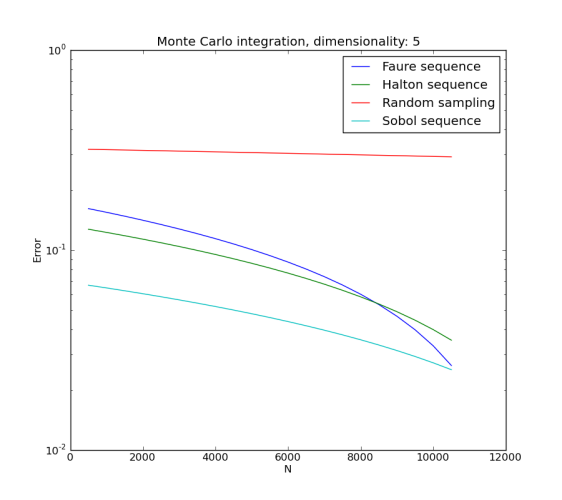
The monteCarloIncremental() function which implements the main work cycle ends here. Next, we call it with two different sets of parameters: first call is a 3-dimensional task with 20 points added per step and a maximum of 1000 point total, second is a 5-dimensional task with 500 points per step and a maximum of 15 000 points:

if __name__ == "__main__":
  """
  Example of Monte Carlo integration with GTDoE.
  """
  #3 dimensions, 1000 points
  monteCarloIncremental(3, 1000, 20)

  #5 dimensions, 15000 points
  monteCarloIncremental(5, 15000, 500)

To run the example, open a command prompt and execute:

python -m da.p7core.examples.gtdoe.example_gtdoe_montecarlo

You can also get the full code and run the example as a script: example_gtdoe_montecarlo.py.

Running the example will perform the two tasks described above and display a convergence graph for each (when running, close the window displaying the first graph to proceed to the second task). The plots show that convergence of the considered integral is much faster with sequential GTDoE techniques than with plain random sequence:

More GTDoE examples can also be found in Code Samples.