1.1. Optimization

1.1.1. Introduction

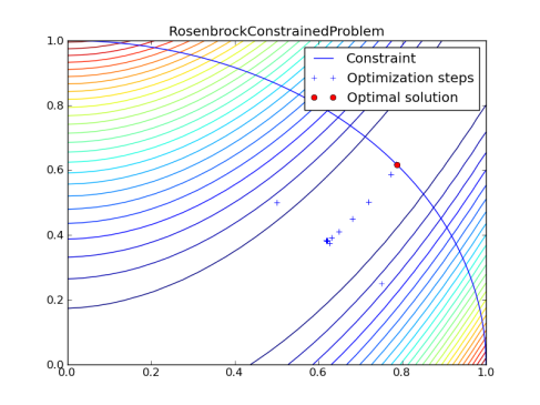
This example shows how to use pSeven Core to find the minimum of the Rosenbrock function with an imposed constraint:

\begin{eqnarray} &f(\mathbf{x}) = 100 (x_1 - x^2_0)^2 + (1 - x_0)^2 \\ &x_0^2 + x_1^2 \leq 1 \end{eqnarray}

Start by importing the Generic Tool for Optimization (GTOpt) module:

from da.p7core import gtopt

1.1.2. Problem Definition

To define the problem, you have to implement your problem class, inherited from one of GTOpt’s problem classes. Since there is a constraint in the problem, inherit from ProblemConstrained.

class RosenbrockConstrainedProblem(gtopt.ProblemConstrained):

Implement prepare_problem() to describe variables and objectives.

def prepare_problem(self):

Add variables using add_variable(). The design space is 2-dimensional: \(0 \leq x_i \leq 1,\ i = 1,2\). The variable bounds (also called box bounds) are due to the constraint — there is no need to search for a solution in those design space regions which clearly violate the constraint. Note that you should specify an initial guess for each variable (\(0.5\) for example).

self.add_variable((0, 1), 0.5)
self.add_variable((0, 1), 0.5)

Add an objective using add_objective().

self.add_objective()

Add the constraint with add_constraint(). This method only declares that there is a constraint in the problem and sets the constraint bounds. Constraint definition is given in define_constraints(). Here, add_constraint() also specifies a hint, which informs optimizer of the constraint type (see Hint Reference).

self.add_constraint((0., 1.), hints = {'@GTOpt/LinearityType': 'Quadratic'})

Finally, enable saving evaluation history.

self.enable_history()

This will store variable, objective and constraint values obtained while solving in problem’s history. The example uses this data to plot the optimization trajectory later.

Constraint definition:

def define_constraints(self, x):
  return x[0] * x[0] + x[1] * x[1]

Next definition to implement is define_objectives(). It contains the actual formula calculating the objective:

def define_objectives(self, x):
  return 100.0 * (x[1] - x[0]*x[0])*(x[1] - x[0]*x[0]) + (1.0 - x[0])*(1.0 - x[0])

Now you have a class that describes the Rosenbrock problem:

class RosenbrockConstrainedProblem(gtopt.ProblemConstrained):

  def prepare_problem(self):
    self.add_objective()
    self.add_constraint((0., 1.), hints = {'@GTOpt/LinearityType' : 'Quadratic'})
    self.add_variable((0, 1), 0.5)
    self.add_variable((0, 1), 0.5)
    self.enable_history()

  def define_constraints(self, x):
    return x[0] * x[0] + x[1] * x[1]

  def define_objectives(self, x):
    return 100.0 * (x[1] - x[0]*x[0])*(x[1] - x[0]*x[0]) + (1.0 - x[0])*(1.0 - x[0])

1.1.3. Solver Setup

To set up optimization, create a gtopt.Solver instance:

optimizer = gtopt.Solver()

You can set a logger (see Loggers) and a watcher (see Watchers), and also change solving options (see Options Interface).

Begin with the logger. Import StreamLogger and create its instance which will write to stdout at the debug log level. Attach the logger using set_logger():

import sys

from da.p7core import loggers

debug_stdout_logger = loggers.StreamLogger(sys.stdout, loggers.LogLevel.DEBUG)
optimizer.set_logger(debug_stdout_logger)

A watcher is a callable object that is called by the optimizer once in a while. If the watcher returns False, optimizer interrupts the problem solving. For this example, implement a simple watcher which always returns True:

class CustomWatcher(object):
  def __call__(self, obj):
    return True

Create a CustomWatcher instance and connect it to the optimizer using set_watcher():

simple_watcher = CustomWatcher()
optimizer.set_watcher(simple_watcher)

Now, since the logger works at the debug level, you need to configure the solver so it provides the debug information to logger: set the GTOpt/LogLevel option to "Debug" (its default is "Info"):

optimizer.options.set('GTOpt/LogLevel', 'Debug')

1.1.4. Solving the Problem

Create an instance of the RosenbrockConstrainedProblem class:

problem = RosenbrockConstrainedProblem()

You can print a readable problem summary:

print(problem)

Solve the problem and get the result:

result = optimizer.solve(problem)

Print a readable result summary:

print(result)

Print the optimum point:

print("Optimal x: %s" % result.optimal.x)
print("Optimal f: %s" % result.optimal.f)

1.1.5. Full Example Code

Finally, putting it all together gives:

import sys

from da.p7core import gtopt
from da.p7core import loggers


class RosenbrockConstrainedProblem(gtopt.ProblemConstrained):

  def prepare_problem(self):
    self.add_objective()
    self.add_constraint((0., 1.), hints = {'@GTOpt/LinearityType' : 'Quadratic'})
    self.add_variable((0, 1), 0.5)
    self.add_variable((0, 1), 0.5)
    self.enable_history()

  def define_constraints(self, x):
    return x[0] * x[0] + x[1] * x[1]

  def define_objectives(self, x):
    return 100.0 * (x[1] - x[0]*x[0])*(x[1] - x[0]*x[0]) + (1.0 - x[0])*(1.0 - x[0])

class CustomWatcher(object):
  def __call__(self, obj):
    return True

optimizer = gtopt.Solver()

info_stdout_logger = loggers.StreamLogger(sys.stdout, loggers.LogLevel.DEBUG)
optimizer.set_logger(info_stdout_logger)
optimizer.options.set('GTOpt/LogLevel', 'Debug')

simple_watcher = CustomWatcher()
optimizer.set_watcher(simple_watcher)

problem = RosenbrockConstrainedProblem()
print(problem)
result = optimizer.solve(problem)
print(result)
print("Optimal x: %s" % result.optimal.x)
print("Optimal f: %s" % result.optimal.f)

The solution may be visualized using Matplotlib. Here we provide an example of how this may be done; note it requires matplotlib version at least 1.1 to be displayed correctly.

import matplotlib.pyplot as plt
import numpy as np

import os
import math

plt.clf()
fig = plt.figure(1)
title = problem.__class__.__name__
plt.title(title)

# Rosenbrock function levels
x = y = np.linspace(0, 1, 30)
[X, Y] = np.meshgrid(x, y)
Z = 100.0 * (Y - X*X)*(Y - X*X) + (1.0 - X)*(1.0 - X)
plt.contour(X,Y,Z, 30)

# constraint curve
cx1 = np.linspace(0., 1., 1000, True)
cx2 = np.sqrt(1.0-cx1*cx1)
plt.plot(cx1, cx2, label = 'Constraint')

history = np.array(problem.history, dtype=np.float)
plt.plot(history[:, 0], history[:, 1], 'b+', label = 'Optimization steps')
plt.plot(result.optimal.x[0][0], result.optimal.x[0][1], 'ro', label = 'Optimal solution')
plt.legend()

fig.savefig(title)
print('Plots are saved to %s.png' % os.path.join(os.getcwd(), title))
if not os.environ.has_key('SUPPRESS_SHOW_PLOTS'):
  plt.show()

On the plot you see the optimization steps (note the initial guess point at \([0.5, 0.5]\)) and the solution point. It also shows Rosenbrock function level lines and the egde of feasibility region.