3.8. Surrogate Based Optimization

This page discusses the special type of solving algorithms implemented in GTOpt — surrogate based optimization (SBO).

3.8.1. SBO in GTOpt

Surrogate based optimization plays a significant role in GTOpt. SBO algorithms are substantially different from other optimization algorithms. Respective SBO capabilities cover all problems listed in Supported Problem Types, including their robust formulations (see Robust Optimization).

New in version 1.10.2: full support for multi-objective problems.

Prior to 1.10.2, GTOpt allowed only one expensive objective even in multi-objective problems. pSeven Core 1.10.2 implemented the support for multiple expensive objectives, and currently a problem may include any number of expensive objectives and constraints.

New in version 3.0: provides mixed-integer optimization support.

Moreover, since MACROS 3.0 SBO provides the base for mixed-integer variables support in GTOpt (see section Mixed Integer Variables). Formally, SBO methods are invoked for any input problem, which is known to be computationally expensive, however, there are special cases when surrogate modeling is used for cheap to evaluate problems as well.

3.8.2. Overview

Surrogate based optimization in GTOpt is based upon Gaussian processes (GP) modeling technique and originates in well known “Probability of Improvement” (PI) approach. However, GTOpt implements numerous tweaks and changes with respect to conventional formulations, that it is now hardly possible identify GTOpt SBO optimization stack as being GP-based PI methodology. In particular, even GP construction and philosophy have been drastically altered, so that it makes sense to start with qualitative review of corresponding aspects of GTOpt.

Deficiencies of conventional surrogate based optimization approaches could best be illustrated on the example of well known GP modeling. There are essentially two prime weak points, which limits its applicability:

1. Model training takes prohibitively large time and has large memory footprint.

   Indeed, model training implies maximization of some derived quantity, usually likelihood or some cross validation criterion. In either case, it reduces to multiple evaluation of model predictions with varying model parameters, which implies in turn the need to invert the correlation matrix on every parameters change. With usual implementation the cost of every evaluation scales like \(O(N_{sample}^3)\) (\(N_{sample}\) being the current sample size) because the correlation matrix is of size \(N_{sample} \times N_{sample}\) and becomes computationally prohibitive already for moderate samples \(N_{sample} \sim O(10^3)\). In problems with large dimensional design scape situation is even worse because of the large number of involved model parameters. Indeed, the minimal required number of sampled designs scales like \(N_{sample} \sim N\) in \(N\) dimensions, total number of model parameters to be determined is of the same order, \(N_{param} \sim N\). Moreover, the number of iterations required to locate likelihood maximum is again of order \(N\), \(N_{iter} \sim N\), each of which costs \(N\) evaluations at different parameters values. Overall conclusion is that the cost of model training scales with problem dimensionality as

   \[N_{iter} \cdot N \cdot N^3_{sample} \sim N^5\]

   In a nutshell, the above implies that conventional GP-based SBO strategies are not applicable to large scale problems. It is true that recently there were a few notable algorithmic achievements, aimed to overcome these limitations, for instance, for large samples one could exclusively utilize iterative matrix methods and thus reduce the cost of every elementary step to \(O(N_{sample}^2)\). Although this helps to push maximal manageable sample sizes to something like a few thousands, this solution is not entirely satisfactory, we simply change the above \(N^5\) estimate to something like \(N^4\), which is still prohibitive at large \(N\).

2. None of conventional surrogate models properly takes into account possible multi-scale dependencies of underlying model.

   Here we mean primarily the fact, that virtually all the surrogate models used nowadays have only a small number of tunable parameters. Hence, they cannot be adequate for models, which exhibit multi-scale behavior. The need to invent multi-resolution models had become evident long ago (see, for instance, recent activities in this field in mathematical statistics literature), however, we are not aware of any satisfactory solution up to now. Note that the wish to have multi-resolution surrogates contradicts previously discussed complexity of model construction process: the more parameters surrogate model possess (multi-resolution) the more costly it becomes to construct (training time).

To summarize, the need to apply SBO inspired techniques to large scale problems requires to resolve two contradictory issues: reduce to admissible level the cost of model training (both the time and memory requirements) and simultaneously incorporate multi-resolution capabilities into the model, because generically high dimensional underlying models do exhibit different length scales.

Although the above challenge might seem unsolvable, there is a crucial simplifying observation. Namely, we are not going to construct full fledged surrogate models for underlying responses as it is usually the goal in mathematical statistics. In optimization context the goal is to find optimal solution and not to predict responses away from optimality. This means, in particular, that surrogates must be accurate only in promising regions of the design space. Technically, this might be best illustrated by the generic sequence of steps performed during surrogate-based optimization (SBO). Here, one starts with initial design of experiment (DoE) plan aimed to produce well separated set of points having good space filling properties. By its very definition, DoE generated sample is almost uniform in the design space and therefore there is a single number characterizing DoE sample: characteristic (mean) distance \(L_{mean}\) between nearest designs. Suppose now that we want to train GP model on DoE generated sample. Silent feature of virtually any GP model is that its tunable parameters reflect the correlation lengths along different coordinate axes in the design space. Then it follows just from dimensional analysis that properly trained GP model ought to have tuned parameters equal to \(L_{mean}\) up to dimensionless factors of order one. An immediate and surprising conclusion is that model training is in fact redundant once training set is uniformly distributed and has single characteristic length scale: optimal parameter values at least in case of Kriging-like GP models might be guessed a priori without any actual likelihood optimization. To be on the safe side, one should, of course, check the adequacy of guessed optimal parameters and, perhaps, perform a few likelihood optimization steps. However, this does not invalidate the prime message of performed analysis: full fledged likelihood optimization should not be conducted, relevant surrogate model parameters might be guessed in advance.

The above conclusion is a great step towards reducing the cost of surrogate model training. However, it is operational only at the initial DoE stage and seems to be not applicable after that. To proceed, we need to consider (in general terms) the sequence of SBO steps performed to get optimal solution. These are very simple ideologically: given current surrogate model optimizer predicts a few promising locations and evaluates underlying model at these designs. Then training set is augmented with newly discovered responses, surrogate model is retrained and optimization process proceeds to the next iteration. Prime observations here:

1. New designs are added at distinguished locations only, hopefully, near the (locally) optimal solution.
2. Only a few designs are added at a time (number of added designs is much smaller than the current sample size).
3. Characteristic nearest neighbor distances in the vicinity of added designs is smaller than that of original sample.

It follows then that initial DoE sample is in fact augmented with well-localized clusters of new solutions. Qualitatively, upon accounting for new designs surrogate models should only change in the vicinity of added points, far away from added clusters surrogate are expected to remain intact. Moreover, due to relatively small distance scale within each cluster compared to that of underlying sample correlations within each cluster are expected to be stronger than that between new solutions and points from current sample. Thus we should explicitly account for correlations within each cluster. Moreover, each of these in-cluster correlations are to be described by new cluster-specific GP models, ultimate reason being that distances within each cluster are small and hence corresponding responses might experience multi-resolution properties of underlying model.

In more detail, the above reasoning might be reduced to the following formulation:

1. Evaluated designs eventually cluster in promising regions of the design space.

2. Hierarchy of length scales could be observed:

   Let \(\langle L_x \rangle\) denote a characteristic distance between nearest sampled designs around \(x\). Then:

   • DoE stage: \(\langle L_x \rangle = L_0 \quad \forall x\)

   • After a few iterations (\(\Omega\) is some promising region):

     \[\begin{split}\begin{array}{ll} \langle L_x \rangle = L_0 & x \notin \Omega \\ \langle L_x \rangle = L_1 & x \in \Omega \\ L_1 ~ \lesssim ~ L_0 & \end{array}\end{split}\]

   • At later stages (\(\Omega_i\) are the nested promising regions):

     \[\begin{split}\begin{align*} \langle L_x \rangle = L_0 & \quad x \notin \Omega \\ \langle L_x \rangle = L_1 & \quad x \in \Omega_1 \\ & \cdots \\ \langle L_x \rangle = L_k & \quad x \in \Omega_k \\ L_k \lesssim \cdots & \lesssim L_1 \lesssim L_0 \end{align*}\end{split}\]

Therefore, at the expense of additional evaluations we enforce length scales hierarchy at every iteration: instead of single candidate evaluation we perform DoE sampling in candidate’s vicinity, determined by upper region length scale. Consequences:

• Underlying model is not only probed at candidate location \(x_c\), but is explored in candidate’s vicinity \(\Omega(x_c)\).

  \[F(x_c) ~\to ~ \{ F(x_i) \}, \, i \in \Omega(x_c)\]

• Every iteration induces well-defined smaller length scale \(L_k\)

  \[L_k \lesssim \cdots \lesssim L_1 \lesssim L_0\,,\]

  each \(L_k\) being associated with particular nested regions.

As a crucial side effect of the above reasoning we note that for each new submodel the training process becomes essentially simple as it was for the first model constructed at DoE stage. The only thing which is yet to be discussed is how to unify various surrogates into one global model describing underlying responses in whole design space. For only one added cluster the answer seems to be simple: in addition to correlations \(K^{(0)}(x,y)\), present before new solutions were added, additional contribution looks like composition of three terms:

1. From point \(x\) to some clustered design \(z_i\).
2. Within new cluster correlations of points \(z_i\) and \(z_j\).
3. From point \(z_j\) to considered location \(y\).

Formally, updated correlation function looks like:

\[K(x,y) ~=~ K^{(0)}(x,y) ~+~ \alpha \, \sum_{i,j} K^{(1)}(x,z_i) \,[K^{(1)}]^{-1}(z_i,z_j) \, K^{(1)}(z_j,y)\]

where the only undetermined parameter is the relative magnitude of new correlations with respect to old ones. This is important: the above generic reasoning valid in SBO context lead us to the conclusion that surrogate model updating reduces to simple one-dimensional optimization subproblem to determine relative weight factor \(\alpha\). All other parameters are determined a priory thanks to the specific design space resolution properties of SBO methodology.

The above construction trivially generalizes to the case of several nested regions in which separate GP models are defined. Namely, ansatz for multi-resolution GP correlation function, which reflects the above hierarchy of length scales, reads

\[K(x,y) ~=~ K^{(0)}(x,y) ~+~ \sum_\mu ~ \alpha_\mu ~ \sum_{i,j} ~ K^{(\mu)}( x, x^i_\mu) ~ [K^{(\mu)}]^{-1}_{ij} ~ K^{(\mu)}( x^j_\mu, y )\,,\]

where \(K^{(\mu)}\) are \(\Omega_\mu\)-specific correlation vector/matrix. Parameters to be determined here include only relative amplitudes \(\alpha_\mu \ge 0\).

To summarize, our proposition is to radically reduce the computational cost of surrogate-based optimization simultaneously introducing multi-resolution capabilities into the surrogate models. Underlying idea is based on the specifics of virtually any SBO setup, namely, the fact that uniformity of sampled designs could easily be achieved at every SBO step. Price to pay is the necessity to explicitly maintain the hierarchy of surrogate models, each describing subsample correlations at every SBO step. However, this should be considered as advantage, not the drawback: hierarchical structure of surrogates naturally admits multi-resolution capabilities of total surrogate model. Prime distinctive features of our approach:

• Prime gross features of every correlation function \(K^{(\mu)}\) are known in advance once length scale hierarchy is respected.
• Seems that one could avoid \(K^{(\mu)}\)-parameters tuning (“training”) altogether.
• Only amplitudes \(\alpha_\mu\) are to be determined for every new region (every iteration).
• \(\alpha_\mu\) determination is cheap (no inversions of large matrices is involved).
• Knowledge of length scale hierarchy allows to predict the domains where model is changing upon the sample augmentation.

3.8.3. Single-Objective Constrained SBO

We have to distinguish two vastly different cases:

1. Expensive objective function (perhaps, supplemented with cheap constraints).
2. Single expensive constraint entering the problem with cheap objective function.

Generic combination of cheap/expensive observables is a natural generalization of these two extremes. Let’s consider the first case first.

The case of single expensive objective function.

Our approach is modeled around the well-known “Probability of Improvement” treatment, in which auxiliary internal subproblem to be solved reads

\[x^* = \mathrm{arg} \max_x PI(x) \qquad PI(x) = \Phi[u] \qquad u = \frac{f^* - \hat{f}_x}{\hat{\sigma_x}}\]

where \((\hat{f},\hat{\sigma})\) is the surrogate model prediction and uncertainty. Note that numerically it is complete disaster to consider \(\Phi[u]\). Instead GTOpt solves equivalent problem

\[x^* = \mathrm{arg} \max_x \, u_x\]

Meaning of PI criterion is simple: solution \(x*\) is the point at which probability to improve current best value \(f^*\) is maximal (including prediction uncertainties). There are a few weak points of PI strategy:

• Performance crucially depends upon the choice of \(f^*\) value. Indeed, \(f^*\) is to large extent arbitrary, there are two limiting cases:
  • \(f^* = -\epsilon + \min \hat{f}\): algorithm often “hangs” in small vicinity of already known solutions.
  • \(f^* = -\infty\) : algorithm essentially find \(x^* = \mathrm{arg}\max \hat{\sigma}\), which is a badly posed problem (multiple equivalent solutions).
• Algorithm is not sufficiently robust with respect to (hopefully, small) inadequacy of surrogates. When surrogate model predictions deviate significantly from true responses PI criterion suggests wrong evaluation candidates.

To ameliorate both the above deficiencies GTOpt considers “continuous” family of PI-like criteria \(PI(x, t)\):

\[f^* ~\to ~ f^*(t) = -t\, |\Delta f| ~+~ \min \hat{f} \qquad t \in [0:1]\]

where \(\Delta f\) is estimated range of objective function variation and is chosen such that \(t \in [0:1]\) provides a homotopy between local and global search modes. The solution \(x^*\) also becomes \(t\)-dependent

\[x^* ~ \to ~ x^*(t)\]

and it is crucial to investigate the continuity of the path \(x^*(t)\) in the design space. Note that the above mentioned switch from local to global search with rising \(t\) manifests itself in discontinuity of \(x^*(t)\) at some t-values

\[x^*(t_i - 0) \ne x^*(t_i + 0)\]

Technically, we consider sufficiently large number of \(t\)-values:

• Discontinuity of \(x^*(t)\) is revealed by the appearance of several well-separated clusters of evaluation candidates.
• Within each cluster we could pick up essentially any point as the next candidate to be evaluated.

The above ensures the presence of both local and global search modes in GTOpt SBO strategy. Overall algorithm performance crucially depends upon the solution of internal auxiliary problem. We utilize multi-start strategy which gradually reaches optimal solution and allows to keep candidates to be reused on next SBO iterate:

• Take sufficiently large number of initial guesses and sufficiently crude termination tolerances.
• Push current candidates towards local optimal solutions.
• Cluster resulting set and select only one candidate from each cluster.
• Diminish termination tolerances and close the cycle.

Note: intermediate locally optimal designs are the natural candidates for multi-starts at next SBO iteration thanks to multi-resolution capabilities of utilized surrogate models.

It remains to discuss how the surrogate models are updated during the course of algorithm. Normally, underlying model is evaluated for each obtained evaluation candidate \(x^*_i\), surrogates are updated with new responses. However, implemented hierarchical GP appeal to slightly different strategy, which requires the following actions for each candidate point \(x^*_i\):

• Establish local characteristic length scale \(\lambda_i\) between nearby sampled designs.
• Generate DoE plan in the vicinity of \(x^*_i\) with characteristic length scale \(\bar{\lambda}_i < \lambda_i\).
• Evaluate underlying model at generated locations. These responses are to be used to train next hierarchical GP level.

The case of single expensive constraint and cheap objective function.

Consider the case of cheap objective supplemented with one expensive constraint

\[\min_x f \qquad c_L \le c \le c_U\]

for which current surrogate model \(\hat{c}\) is available. GTOpt establishes next evaluation candidate in two stages:

1. Solve

   \[\min_x f \qquad c_L \le \hat{c} \le c_U\]

   infeasibility of which says nothing about infeasibility of original problem. If it is infeasible, design with minimal constraints violations is taken as \(x^*\).

2. Otherwise, GTOpt takes into account model uncertainties by considering

   \[\min_x f \qquad \Phi\left[\frac{c_L - \hat{c}}{\hat{\sigma}}\right] \le \alpha \qquad \Phi\left[\frac{\hat{c} - c_U}{\hat{\sigma}}\right] \le \alpha\]

   with predefined small \(\alpha\)-parameter (quantile).

3.8.4. Multi-Objective Constrained SBO

Multi-Objective SBO optimization of GTOpt is build on top of corresponding single-objective counterpart, hence directly utilizes all the advantages of respective algorithms (see above). We only need to overview how the original multi-objective problem is reduced to the sequence of single-objective treatments. Underlying idea is simple: first, GTOpt establishes complete set of anchor points in close analogy to what is done in non-surrogate based approaches (see Multi-Objective Optimization for details). Anchor points determination allows to estimate global geometry of Pareto frontier, to detect degenerate cases earlier and to proceed to the second stage of Pareto frontier discovery.

Second stage utilizes the notion of Chebyshev convolution to construct particular instance of single-objective problem, the solution of which provides new Pareto optimal design. In more detail, respective single objective function looks like:

\[\max_i [ \alpha_i \cdot f_i ] \quad \sum_i\alpha_i = 1 \qquad i = 1, ..., K\]

where the coefficients \(\alpha_i\), parameterizing \(K\)-dimensional simplex, are varied from iteration to iteration in a way, which ensures even coverage of Pareto frontier.

3.8.5. Parallel SBO

Usually the prime criterion to estimate the efficiency of a particular SBO algorithm is the number of evaluations needed to attain the given “acceptable” level of optimized objective function. Arguments here are simple: for virtually all engineering applications every function evaluation is quite expensive computationally and thus the ultimate goal is to reduce the required evaluation count as much as possible.

However, recent rapid development of high-performance computing power greatly challenges (and even invalidates) this simple efficiency model. Indeed, nowadays computer clusters, which could do many computational jobs in parallel, are widely available. It then makes sense to ask: what is the suitable meaning of “evaluation count” in parallel environment, which can perform \(N_{batch} \gt 1\) jobs simultaneously?

One rather attractive in many contexts viewpoint asserts that plain “total evaluation count” \(N_{eval}\) does not really matter, rather the significant quantity to reduce total modeling time is the total number of performed batch calls (“batch evaluation count”) \(N^{batch}_{eval}\), each consisting of no more than \(N_{batch}\) “elementary” evaluations which are expected to be done in parallel. This performance criterion is quite natural and explicitly alludes to parallelization capabilities of particular optimizer. Indeed, nowadays parallelization is the prime approach to boost the performance of virtually any software. However, in the optimization context there is an additional subtlety, which must be discussed. Point is that optimization and parallelization are mutually inconsistent: wise algorithms are not really parallelizable, while silly methods allow almost perfect parallelization (think about two extreme cases: random search, which admits perfect parallelization, and an ideal optimizer, which finds optimal solution at once). Therefore, only imperfect optimization algorithms could ever benefit from concurrent evaluations. Hopefully, none of methods are perfect and there are always some room to boost performance in parallel environment. Degree of success of parallelization depends strongly upon the particular method, however, some general estimates might be given. For instance, performance of the majority of well known optimization algorithms indeed boosts significantly for \(N_{batch} \lesssim N\) (dimensionality of the considered problem), while for larger batch sizes performance curve evidently flattens. Therefore, one might expect rather generically that characteristic batch size for which performance might yet rise is of order problem dimensionality, larger batch sizes are not worth to consider.

Below we illustrate that performance of SBO algorithms indeed rises in parallel environment for expected range of the batch size, \(N_{batch} \le N\). Example problem to consider is the well known Levy function defined in hypercube \([-10, 10]^{20}\). The following figure represents the best attained objective value as a function total number of evaluations for various indicated batch sizes (initial DoE volume is about 250 and is insignificant).

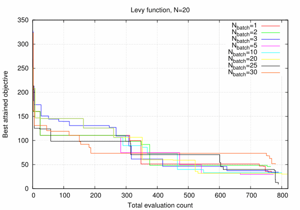
It can be seen that performance with respect to the total number of evaluations does not change with batch size despite the fact that many evaluations had been performed in parallel. However, situation changes radically when we plot best attained objective value versus the number of batch evaluations.

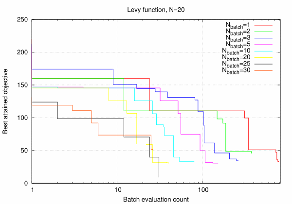
Evidently, performance defined this way rises almost linearly with \(N_{batch}\) signifying almost perfect parallelization efficiency up to \(N_{batch} \sim N\). For larger batch sizes parallelization efficiency degrades as is seen from the curves for \(N_{batch}\) 25 and 30.

3.8.6. High-Dimensional SBO

One important feature of surrogate-based optimization algorithms is that they are operational in large dimensional design spaces. How large the characteristic maximal dimensionality might be and why usual (say, GP-based) approaches cannot properly address these problems?

There are essentially two prime reasons. One is the prohibitive computational complexity of model training process. Indeed, in \(D\) dimensions minimal reasonable training sample size is of order

\[N_{DoE} \sim D^\alpha, ~ \alpha \in [1:2].\]

Since the number of (hyper)-parameters to be selected during the training process is no less than \(D\), the total computational complexity, measured in CPU time spent, scales at least like

\[T_{train} \sim D^2 D^{3\alpha} \gtrsim D^5,\]

where \(D^{3\alpha}\) is the cost of single correlation matrix inversion and \(D^2\) is the minimum number of evaluations required to get optimal solution in \(D\) dimensions. Thus, usual GP-based SBO approaches are not really operational in more than \(D \sim 50\) dimensions due to the rapidly rising computational complexity.

Second important difficulty comes from the computational cost of making optimal points predictions using already trained surrogate model. Indeed, single local optimization over constructed surrogate takes \(\sim D^2 D^{2\alpha}\) operations, where the first factor is the cost of single local optimization and the second one is the (optimistic) estimate of single model response evaluation. However, it is crucial that in usual circumstances model training is a global process meaning that upon re-training model might change in all the design space. Moreover, in absolute majority of cases surrogates exhibit significant multi-modal behavior and hence require globalized treatment. Therefore, in order to get proper optimal point prediction one has to perform at least \(\sim N_{DoE} \sim D^\alpha\) local optimizations, which boosts the total computational cost up to

\[T_{predict} \sim D^2 D^{3\alpha} \gtrsim D^5\]

which is essentially of the same order as the training complexity.

Purpose of this section is to demonstrate that GTOpt specific SBO methods do not exhibit the above prohibitive scaling law and remain practical at least up to \(D \sim 100\). Moreover, even the total time required to perform optimization scales negligibly compared to \(D^5\) rule thanks to in-house developed multi-resolution GP-based surrogate modeling. This is achieved due to the following reasons:

1. Careful preparation of DoE sample allows to reduce initial training time to \(T_{train} \sim D^0\). The trick is provided by the fact that DoE sample is taken coherent with respect to nearest-neighbors separations and hence allows to guess rather precisely appropriate hyper-parameters a priori.
2. At latter stages sample coherence is always maintained: new designs are selected in a specific distance-coherent fashion and do not spoil the coherence of already accumulated sample (this is the essence of multi-resolution).
3. As a consequence, upon re-training model changes in well localized regions of the design space, which greatly facilitates its forthcoming global optimization. Note however that model optimization complexity remains the prime bottleneck since it yet scales like \(T_{predict} \sim D^2 D^{2\alpha} \gtrsim D^4\) (\(D^\alpha\) gain is because full-fledged global optimization is not needed anymore).

To illustrate the above we consider well-known Levy function in hypercube \([-L, L]^D\), the volume of which remains roughly constant as design-space dimensionality \(D\) is increased. The reason is that at constant \(L\) complexity of considered case rises exponentially with \(D\), but we want to have it approximately constant. Note that precise definition of used test function is not important anyway, we are not going to compare SBO efficiency at various \(D\).

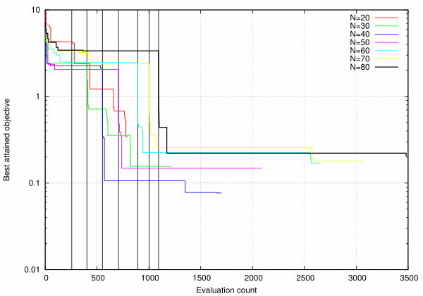
The above figure represents optimization history (best attained objective) as a function of total evaluation count at various design space dimensionality. In all considered cases the same default options had been used. Note that DoE and total sample volumes differ at different \(D\) (corresponding dependency has been discussed above), for each dimensionality we added solid vertical line to indicate respective DoE sample size (it rises monotonically with \(D\)). It can be seen GTOpt SBO algorithms flawlessly handle samples as large as \(\sim 4 10^3\) and exhibit no significant performance degradation.

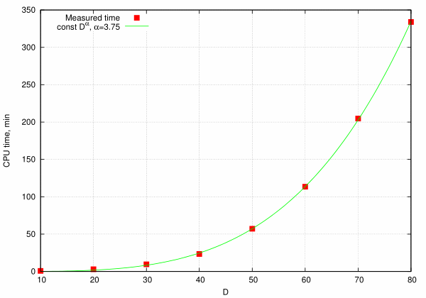
As far as complexity scaling is concerned, we plot total CPU time spent to solve the problem versus problem dimensionality (red points) together with best power-like fit (green line). Data clearly confirms power-like scaling of method complexity with exponent being only slightly less than was predicted above (\(\alpha = 3.75\) with “theoretical” value 4).

3.8.7. Direct SBO

As described above (see Single-Objective Constrained SBO), the general SBO framework deals with the exploration-exploitation trade-off by optimizing a special criterion that takes both the value and the uncertainty of a surrogate model.

However, the exploration may not always be necessary or affordable in some engineering problems, yet the global search stable to noise is still required. For such situations, we provide a Direct SBO approach that essentially relies only on the exploitation meaning that it takes into account only the value of a surrogate model.

In case with Direct SBO, it is expected that the applied criterion is fitted into the general SBO scheme: it starts from DoE stage, then constructs surrogate models, then updates models using responses of observables in optimal points predicated by the surrogate models.

This approach can be useful for constrained or multi-objective optimization when non-trivial trade-offs between different expensive to evaluate observables need to be found.

Direct SBO can be enabled by setting GTOpt/GlobalPhaseIntensity to zero.

3.8.8. Summary

Surrogate based optimization in GTOpt provides an universal set of algorithms aimed to deal with virtually any expensive input problems, ranging from simplest unconstrained single-objective case to the most difficult to handle multi-objective robust formulations. It incorporates cutting-edge efficient methods for both the surrogate models construction and their forthcoming exploration. Prime advantage of surrogate modeling in GTOpt is its multi-resolution ability, which being supplemented with specific hierarchical optimization strategies, allows to address large-scale expensive optimization problems, which are difficult to consider with conventional methods.