12.2. GTOpt

12.2.1. Multi-Objective Optimization

One of the distinctive features of GTOpt is the support for multi-objective optimization. This example demonstrates the approach to multi-objective optimization problems with GTOpt by solving the ZDT1 problem:

\begin{eqnarray} &g(\mathbf{x}) = 1 + \frac{9}{n-1}\sum_{i=2}^n x_i \nonumber \\ &f_1(\mathbf{x}) = x_1 \nonumber \\ &f_2 = g(\mathbf{x})\left(1-\sqrt{\frac{x_1}{g(\mathbf{x})}}\right) \nonumber \\ &0 \le x_i \le 1 \nonumber \end{eqnarray}

We will consider the case of \(n = 2\), so the actual definition looks as follows:

\begin{eqnarray} &f_1(\mathbf{x}) = x_1 \nonumber \\ &g(\mathbf{x}) = 1 + {9}{x_2} \nonumber \\ &f_2 = g(\mathbf{x})\left(1-\sqrt{\frac{x_1}{g(\mathbf{x})}}\right) \nonumber \\ &0 \le x_i \le 1 \nonumber \end{eqnarray}

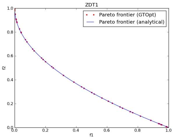
The Pareto frontier for ZDT1 problem is known to be \(f_2 = 1 - \sqrt{f_1}\). The results obtained by GTOpt will be plotted over this curve to illustrate the solution quality (note it requires Matplotlib version at least 1.1 to be displayed correctly).

ZDT1 is an unconstrained two objective problem, so we will have to inherit our problem from the ProblemUnconstrained class and define its properties by implementing the prepare_problem() method which will add two variables \(x_1\) and \(x_2\) bound to \([0, 1]\), and the define_objectives() method which will contain the \(g\), \(f_1\) and \(f_2\) function definitions.

Begin with importing modules. Note that this example requires Matplotlib for plotting; it is recommended to use at least version 1.1 to render the plots correctly.

from da.p7core import gtopt
from da.p7core import loggers

import numpy as np
import matplotlib.pyplot as plt

import os

The ZDT1 class which describes the problem:

class ZDT1(gtopt.ProblemUnconstrained):
  def prepare_problem(self):
    self.add_variable((0, 1))
    self.add_variable((0, 1))
    self.add_objective()
    self.add_objective()

  def define_objectives(self, x):
    f1 = x[0]
    g = 1.0 + 9.0 * x[1]
    f2 = g * (1.0 - np.sqrt(f1 / g))
    return f1, f2

Next we will define the problem solving and plotting methods to have a convenient way for invoking the GTOpt solver and processing the results. Solving method which accepts the problem we have just defined as the ZDT1 class looks like follows:

def solve_problem(problem):
  print(str(problem))
  optimizer = gtopt.Solver()
  optimizer.set_logger(loggers.StreamLogger())
  optimizer.options.set('GTOpt/FrontDensity', 15)
  result = optimizer.solve(problem)
  print(str(result))
  print("Optimal points:")
  result.optimal.pprint(limit=10)
  return result

Here, we set up the solver increasing the number of Pareto optimal solutions to be generated by GTOpt by changing the value of the GTOpt/FrontDensity option. This is done merely to obtain more points for the plot and is not essential to get the result. The information about the problem solved and the result will be printed to console. Returned result will be passed to the plotting method which saves an image of obtained Pareto frontier and shows the plot when possible (uses Matplotlib and requires at least version 1.1 to be displayed correctly):

def plot(result):
  fig = plt.figure(1)
  f1, f2 = result.optimal.f.transpose()
  plt.plot(f1, f2, 'bo' , label = 'Pareto Frontier')
  f1_sample = np.linspace(0, 1, 1000)
  plt.plot(f1_sample, 1 - np.sqrt(f1_sample), "r", label='Pareto frontier (analytical)')
  plt.xlabel('f1')
  plt.ylabel('f2')
  plt.legend(loc = 'best')

  title = 'ZDT1 problem'
  plt.title(title)

  fig.savefig(title)
  print('Plots are saved to %s.png' % os.path.join(os.getcwd(), title))
  if 'SUPPRESS_SHOW_PLOTS' not in os.environ:
    plt.show()

The goal here is to quickly provide the visual representation of the result; this method, of course, may be easily adjusted to user needs.

Now that we have defined the above methods, final workflow is very simple. It consists of creating the problem, getting the result from optimizer using the solve_problem() method and displaying it:

def main():
  problem = ZDT1()
  print('=' * 60)
  print('Solve problem %s' % problem.__class__.__name__)
  result = solve_problem(problem)
  plot(result)
  print('Finished!')
  print('=' * 60)

To run the example, open a command prompt and execute:

python -m da.p7core.examples.gtopt.example_gtopt_ZDT1

You can also get the full code and run the example as a script: example_gtopt_ZDT1.py.

Running the example yields an image of Pareto frontier with points showing generated solutions; since we already know the form of the Pareto frontier, we can use this image to assess the quality of GTOpt result:

12.2.2. Surrogate Based Optimization

This example shows how to use surrogate based optimization (SBO). The method is described briefly in the Surrogate Based Optimization section, and details are found in GTOpt manual (see Chapter 4 “Surrogate-Based Optimization (SBO)”).

The example solves a simple unconstrained single-objective problem. The first run, for comparison, does not use SBO. In the second run, the objective is marked expensive, making GTOpt use SBO when solving the problem. Note that the objective function is the same in both runs, and it is not actually expensive:

\begin{eqnarray} &f(\mathbf{x}) = x_1^2 + 4x_2^2 + 8x_3^2 \nonumber \\ &x_i \in (-1, 1) \nonumber \end{eqnarray}

The goal is to demonstrate how the number of evaluation calls is different when using SBO. It does not mean that SBO guarantees a decrease in solving time: due to the overhead of building the surrogate model, total solving time may be more than for a non-SBO solver if the function is not expensive enough — that is, the gain from reducing the number of evaluation calls is not enough to compensate for the overhead, which is clearly visible in this example.

Since the problem is unconstrained, we will inherit its class (SBOSampleProblem) from ProblemUnconstrained and implement the prepare_problem() method to add three variables bound to \([0, 1]\) and one objective. Objective definition (the evaluation function) is given in the define_objectives() method.

Begin with importing modules.

from da.p7core import gtopt
from da.p7core import loggers

import sys

The SBOSampleProblem class which describes the problem:

class SBOSampleProblem(gtopt.ProblemUnconstrained):

  def __init__(self):
    self.count = 0

  def prepare_problem(self):
    self.add_variable((-1, 1), 0.75)
    self.add_variable((-1, 1), 0.75)
    self.add_variable((-1, 1), 0.75)
    self.add_objective()

  def define_objectives(self, x):
    #f = x1^2 + 4*x2^2 + 8*x3^2
    self.count += 1
    return x[0]*x[0] + 4*x[1]*x[1] + 8*x[2]*x[2]

Note it uses a counter for the number of objective function calls. The evaluate() method inherited from ProblemGeneric will call SBOSampleProblem.define_objectives() for evaluation; since the problem includes only one objective, to keep it simple, the counter may be incremented in SBOSampleProblem.define_objectives(). For a generic problem, the increment should be done in evaluate().

Next we define two simple methods for configuring the optimizer and solving the problem:

def optimizer_prepare():
  opt = gtopt.Solver()
  opt.set_logger(loggers.StreamLogger(sys.stdout, loggers.LogLevel.DEBUG))
  opt.options.set({'GTOpt/LogLevel': 'INFO'})
  return opt

def solve_problem(problem, optimizer):
  print(str(problem))
  result = optimizer.solve(problem)
  return result

In the main part, we create two instances of the SBOSampleProblem class, set the expensive objective hint for one of them and solve both problems. Create optimizer:

def main():
  optimizer = optimizer_prepare()

Solve the example problem without using SBO:

  # solve problem not using SBO
  problem = SBOSampleProblem()
  print("\n\nSolving the sample problem without using surrogate based optimization...\n")
  result = solve_problem(problem, optimizer)
  print("\nSolved, wait for SBO version to finish...\n")

Then create the second problem instance, but now mark the objective expensive using the set_objective_hints() method (alternatively, a hint can be set in add_objective(), but it would require to define a second class for this problem):

  # solve the same problem using SBO
  problem_sbo = SBOSampleProblem()
  # define an objective expensive
  problem_sbo.set_objective_hints(0, {'@GTOpt/EvaluationCostType': 'Expensive'})
  # uncomment the following line to obtain the full trace of SBO process (WARNING: this log is about 6 MB size!)
  # optimizer.options.set({'GTOpt/LogLevel': 'DEBUG'})
  print("\n\nSolving the sample problem using surrogate based optimization...\n")
  result_sbo = solve_problem(problem_sbo, optimizer)
  print("\nSolved.\n\nResults:")

Solver info will be logged to the console. For the second problem, the full trace of SBO process may also be obtained by uncommenting the optimizer.options.set({'GTOpt/LogLevel': 'DEBUG'}) line. Note the excessive amount of information; if you do this, it would be better to redirect the logger output.

Print solution (optimal point) and the number of evaluation calls:

  # compare results
  print("=" * 60)
  print("Without SBO.\n")
  print("Optimal point:")
  result.optimal.pprint()
  print("User function calls: %s" % (problem.count))

  print("=" * 60)
  print("Using SBO.\n")
  print("Optimal point:")
  result_sbo.optimal.pprint()
  print("User function calls: %s" % (problem_sbo.count))

  print("=" * 60)
  print("\nFinished!\n")

To run the example, open a command prompt and execute:

python -m da.p7core.examples.gtopt.example_gtopt_SBO

You can also get the full code and run the example as a script: example_gtopt_SBO.py.

Running the example, you can notice that the second problem took much more time than solving without SBO. This is due to the overhead of surrogate models training, mentioned above. However, the number of evaluation calls has decreased significantly: this is the main benefit of surrogate based optimization. This question is discussed in detail in Chapter 4 of the GTOpt user manual.

12.2.3. Batch Mode

This example illustrates the batch mode of GTOpt. It is based on the Multi-Objective Optimization example and solves the same ZDT1 problem, this time in batch mode:

\begin{eqnarray} &f_1(\mathbf{x}) = x_1 \nonumber \\ &g(\mathbf{x}) = 1 + {9}{x_2} \nonumber \\ &f_2 = g(\mathbf{x})\left(1-\sqrt{\frac{x_1}{g(\mathbf{x})}}\right) \nonumber \\ &0 \le x_i \le 1 \nonumber \end{eqnarray}

For comparison purposes, the example defines two different problem classes: the first (ZDT1) is similar to the one found in the example above, while the second (ZDT1Batch) uses the define_objectives_batch() method instead of define_objectives(). Since solutions are the same, they are of no interest here; instead, the example outputs the number of evaluation calls to illustrate the difference between the normal and batch modes.

Begin with importing modules:

from da.p7core import gtopt
from da.p7core import loggers

from pprint import pprint

import sys
from math import sqrt

Define the normal and batch problem classes:

class ZDT1(gtopt.ProblemUnconstrained):

  def __init__(self):
    self.count = 0

  def prepare_problem(self):
    self.add_variable((0, 1))
    self.add_variable((0, 1))
    self.add_objective()
    self.add_objective()

  def define_objectives(self, x):
    f1 = x[0]
    g = 1.0 + 9.0 * x[1]
    f2 = g * (1.0 - sqrt(f1 / g))
    # counter
    self.count += 1
    return f1, f2

class ZDT1Batch(gtopt.ProblemUnconstrained):

  def __init__(self):
    self.count = 0

  def prepare_problem(self):
    self.add_variable((0, 1))
    self.add_variable((0, 1))
    self.add_objective()
    self.add_objective()

  def define_objectives_batch(self, x):
    f_batch = []
    for xi in x:
      f1 = xi[0]
      g = 1.0 + 9.0 * xi[1]
      f2 = g * (1.0 - sqrt(f1 / g))
      f_batch.append([f1, f2])
    # counter
    self.count += 1
    return f_batch

The implementation of define_objectives_batch() in the ZDT1Batch class is in fact similar to the default implementation of this method: it simply loops over a list of requested points, constructing a list of responses. It is assumed that in a real problem the loop is replaced with parallel calls (the example omits this for simplicity).

Define the problem solving method as in the Multi-Objective Optimization example with an additional parameter for the batch mode which sets the value of the GTOpt/BatchSize option:

def solve_problem(problem, batch_size = 1):
  print(str(problem))
  optimizer = gtopt.Solver()
  optimizer.set_logger(loggers.StreamLogger())
  optimizer.options.set({'GTOpt/FrontDensity': 15, 'GTOpt/BatchSize': batch_size})
  result = optimizer.solve(problem)
  return result

Note that all problem classes contain a default implementation of the define_objectives_batch() method, so in fact this method is safe for the ZDT1 problem even with non-default batch size.

In the main part, create instances of the two problem classes and solve them, then print the number of evaluation calls for both:

def main():
  # solve in normal mode

  problem = ZDT1()
  print('=' * 60)
  print('Solve the ZDT1 problem in normal mode.')
  result = solve_problem(problem)
  print(str(result))
  print("\nOptimal points:")
  result.optimal.pprint(limit=10)  # most points omitted to shorten output

  # solve in batch mode, maximum batch size is 10
  problem_batch = ZDT1Batch()
  print('=' * 60)
  print('Solve the ZDT1 problem in batch mode.')
  result_batch = solve_problem(problem_batch, 10)
  print(str(result_batch))
  print("\nOptimal points:")
  result_batch.optimal.pprint(limit=10)  # most points omitted to shorten output

  # print evaluations
  print('=' * 60)
  print('Number of evaluation calls\n')
  print('Normal mode: %s total' % (problem.count))
  print('Batch mode: %s total' % (problem_batch.count))

  print('Finished!')
  print('=' * 60)

To run the example, open a command prompt and execute:

python -m da.p7core.examples.gtopt.example_gtopt_ZDT1_batch

You can also get the full code and run the example as a script: example_gtopt_ZDT1_batch.py.

Running the example outputs problem information and the number of evaluations to the console. As you can see, the total number of evaluations in batch mode is less, because some of them (but not necessarily all) contain multiple points which are needed at the same time for the current optimizer iteration. The number of points requested simultaneously is also not necessarily equal to GTOpt/BatchSize value — it only limits the maximum batch size.

12.2.4. Re-using Evaluation Data in SBO

This example shows how to re-use the evaluation history of previous optimization run in a new one. It considers optimizing the Booth’s function:

\begin{eqnarray} &f(\mathbf{x}) = (x_1 + 2 x_2 - 7)^2 + (2 x_1 + x_2 - 5)^2 \nonumber \\ &-10 \le x_i \le 10 \nonumber \end{eqnarray}

The optimization problem is solved twice. The first time it is solved in usual way. The second time it is solved with data supplied from the first optimization run.

Begin with importing modules:

from da.p7core import gtopt
from da.p7core import loggers

import math
import numpy

Define the problem classes:

class BoothProblem(gtopt.ProblemUnconstrained):
  def prepare_problem(self):
    self.add_variable((-10, 10))
    self.add_variable((-10, 10))
    # define an expensive objective
    self.add_objective(hints = {'@GTOpt/EvaluationCostType': 'Expensive'})

  def define_objectives(self, x):
    return (x[0] + 2 * x[1] - 7)**2 + (2 * x[0] + x[1] - 5)**2

The objective is set expensive because the intention is to involve SBO. Next, set optimizer up:

def main():
  # configure optimizer
  optimizer = gtopt.Solver()
  optimizer.set_logger(loggers.StreamLogger())
  # logging options
  optimizer.options.set({'GTOpt/LogLevel': 'Warn'})
  # limit SBO iterations

  print("*"*90)

  optimizer.options.set({'GTOpt/MaximumExpensiveIterations': 10})
  optimizer.options.set({'GTOpt/GlobalPhaseIntensity': 0})

Note that the number of evaluations is limited here by GTOpt/MaximumExpensiveIterations = 10. Now, solve the problem

  problem = BoothProblem()
  print(str(problem))
  # solve problem using SBO the first time
  result = optimizer.solve(problem)
  print("Initial result %s" % result.optimal.f)
  # all evaluated points are stored in history and can be obtained with designs property
  data = numpy.array(problem.designs)
  print("History 1 %d %s" % (len(data), data))

After optimization is finished the member data designs contains an evaluation history. Data are stored in history in raw format:

\[[x_1, x_N, f_1, \ldots, f_M, c_1, \ldots, c_K].\]

Finally, extract data from history and rerun optimization suppling points and their evaluated responses.

  x = data[:, 0:2]  #x values
  y = data[:, 2]    #x responses
  # resolve the problem with initial data
  problem.clear_history()
  result = optimizer.solve(problem, sample_x=x, sample_f=y)
  print("Improved result %s" % result.optimal.f)
  # Note, that history contains only evaluated points.
  # Points supplied as initial data does not goes to history.
  data = numpy.array(problem.designs)
  print("History 2 %d %s" % (len(data), data))

To run the example, open a command prompt and execute:

python -m da.p7core.examples.gtopt.example_gtopt_SBO_reuse

You can also get the full code and run the example as a script: example_gtopt_SBO_reuse.py.

Running the example outputs problem information, history and results from the first and second runs to the console. You may see that results obtained after the second run improves the results of the first run. It happened because data from the fist run was reused and at the second run SBO was able to construct more accurate models.

Following cases obviously benefit from utilization results of previous optimization:

• Resuming interrupted optimization.
• Increasing evaluation budget after optimization been started.
• Solving modified problem (with other variable or constraint bounds or different cheap objectives or constraints (for the latter corresponding history data have to be alerted))

Suppling initial data to GTOpt also makes sense for gradient-based (cheap) optimization with globalization (GTOpt/GlobalPhaseIntensity > 0).

12.2.5. Surrogate Based Robust Optimization

Here we provide an example that shows how to use GTOpt to solve an optimization problem with uncertanties and a limitation on the number of evaluations of objectives. In this example we suppose that our goal is to find a design that improves the mean (the expectation) of objectives respected some uncontrollable uncertanties. The mean can be estimated by averaging of multiple responses of objectives for the same design. The generic problem statement and general description of approaches are located in the section Robust Optimization.

Such problems always require a lot of total evaluations because, to obtain a reasonable estimation of the mean, a design has to be evaluated many times. So there is no chance to solve such problems for the same limited amount of evaluations as in the basic SBO example (Surrogate Based Optimization). But still there are the number of different approaches that can do adaptive choice for a sample size for averaging and avoid the excessive number of evaluations for designs that are far from optimal thus are capable to save total amount of evaluations.

Two approaches are implemented in GTOpt. The first one relies on smoothness of objectives with fixed value of uncertanties, ability to generate common random numbers and relatively cheap to evaluate objectives. The usage of that approach can be found in example_gtopt_rdo.py .

The second approach, which is used in this example, does not need common random numbers, may work with naturally discrete variables and expect relatively expensive to evaluate objectives. Please, note that for determined problems SBO may work fine when is limited by several hundreds of evaluations, whereas for robust problems to obtain reasonable solution SBO requires thousands (or dozen of thousands in multiobjective case) evaluations.

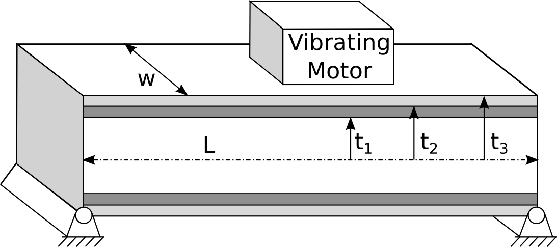
After that brief introduction let us proceed to a problem description. This problem is a modification of Vibrating Platform Design problem from Narayanan, S. and S. Azarm, 1999, “On Improving Multiobjective Genetic Algorithms for Design Optimization” Structural and Multidisciplinary Optimization, 18, pp. 146-155.

We consider a symmetrical five layers platform. The layers of this platform (the inner layer, two middle layers sandwiching the inner layer, and two outer layers sandwiching the inner and middle layers) may be made out of three materials: type \(M_1\), \(M_2\), and \(M_3\). For fixed width and length of the platform, the goal is to choose material types and thickness of layers to minimize the design cost and maximize the vibration frequency of the platform.

The material types differ in physical properties and costs.

	\(M_1\)	\(M_2\)	\(M_3\)
\(\rho\) (\(kg/m^3\))	90 - 100	2493 - 2770	7002 - 7780
E (GPa)	1.44 - 1.6	63 - 70	180 - 200
c (\($/m^3\))	500	1500	800

The range in material properties designates uncertanties in their real quality. For simplicity sake we suppose uniform distribution of uncertanties.

The optimization formulation can be written as following:

\begin{eqnarray} \max_{t, M}&\mathbb{E}_{\xi} f_n(t, \xi) = \left(\frac{\pi}{2L^2} \right) \left(\frac{2w (E_1 t^3_1 + E_2 ( t^3_2 - t^3_1 ) + E_3 ( t^3_3 - t^3_2 )) }{3\mu(t, M, \xi)} \right)^{1/2} \nonumber \\ \min_{t, M}& c(t, M) = 2wL(c_1 t_1 + c_2 ( t_2 - t_1 ) + c_3 ( t_3 - t_2 )) \nonumber \\ &\mu(t, M, \xi) = 2 w (\rho_1 t_1 + \rho_2 ( t_2 - t_1 ) + \rho_3 ( t_3 - t_2 )) \nonumber \\ &\mathbb{E}_{\xi} L \mu (t, M, \xi) \le 2800\\ &0 \le t_2 - t_1 \le 0.15\\ &0 \le t_3 - t_2 \le 0.01\\ &0.05 \le t_1 \le 0.5 \\ &0.2 \le t_2 \le 0.5 \\ &0.2 \le t_3 \le 0.6 \end{eqnarray}

where \(t = t_1, t_2, t_3\) are design variables, \(\xi\) is material uncertainty, \(w, L\) are fixed geometrical parameters of the platform. Value \(\mu\) is linear density of the platform. Values \((\rho_1, \rho_2, \rho_3)\), \((E_1, E_2, E_3)\), and \((c_1, c_2, c_3)\) refer to the density, the modulus of elasticity, and the material cost for the inner, middle, and outer layer of the platform, respectively and depend on discrete variables \(M = (M_1, M_2 ,M_3)\) that determine the choice of materials. The aim is to minimize cost (\(c(t, M)\)) and maximize mean frequency \(f_n(t, M, \xi)\).

Now, we show how to formulate this problem in terms of GTOpt.

First, some modules for GTOpt functionality, problem definition and miscellaneous things have to be imported:

from __future__ import with_statement
from da.p7core import gtopt  # is required for GTOpt functionality
import random  # is required for stochastic problem definition
from math import pi  # is used in objectives definition
import pickle  # is used for exporting raw results
from da.p7core import loggers  # tracks optimizer activity
import matplotlib.pyplot as plt  # depicts results
import os  # is used for determine a path for saving a resulting plot to

Second, we fix a seed to make this example reproduces the same results:

random.seed(111)

It may be removed if reproducibility is not needed.

Third, in order to define GTOpt stochastic problems, the distribution class is defined. If common random numbers variance reduction is used (when all functions are cheap to evaluate), then this class has to be defined specifically. But here it is defined only to satisfy interface:

class Sequential:
  current_value = 0
  def getNumericalSample(self, quantity):
    out = list(range(self.current_value, self.current_value + quantity))
    self.current_value += quantity
    return out
  def getDimension(self):
    return 1

You may note that the class Sequential that defines distribution returns not a random number, but a sequence. This is so because in this example we suppose that stochasticity comes directly from the optimized “black-box”, and it is not possible to allow GTOpt to control random number generator. We will define real stochastic later and here we just tell that each call to “black-box” is unique.

Forth, the optimization problem is defined using GTOpt problem interface class:

class VibratingPlatform(gtopt.ProblemConstrained):
  def __init__(self):
    self.p_def = [100, 2770, 7780]  # kg/m^3
    self.E_def = [1.6, 70, 200]  # GPa
    self.c_def = [500, 1500, 800]  # $
    self.w = 0.4  # m
    self.L = 4.  # m
#[init] end
  def p(self, i):
    i = int(i)
    return self.p_def[i] * (1. - random.random()/10.)

  def c(self, i):
    i = int(i)
    return self.c_def[i]

  def E(self, i):
    i = int(i)
    return self.E_def[i] * (1. - random.random()/10.)
#[matprop] end
  def prepare_problem(self):
    self.add_objective("-freq", hints={"@GTOpt/EvaluationCostType": "Expensive"})
    self.add_objective("cost", hints={"@GTOpt/EvaluationCostType": "Expensive"})

    self.add_variable((0.05, 0.5), name="t1")
    self.add_variable((0.2, 0.5), name="t2")
    self.add_variable((0.2, 0.6), name="t3")

    self.add_variable((0, 2), name="M1", hints={"@GTOpt/VariableType" : "Integer"})
    self.add_variable((0, 2), name="M2", hints={"@GTOpt/VariableType" : "Integer"})
    self.add_variable((0, 2), name="M3", hints={"@GTOpt/VariableType" : "Integer"})

    self.add_constraint((None, 2800.0), hints={"@GTOpt/EvaluationCostType": "Expensive"})
    self.add_constraint((0, 0.15), hints={"@GTOpt/LinearityType" : "Linear"})
    self.add_constraint((0, 0.01), hints={"@GTOpt/LinearityType" : "Linear"})

    self.set_stochastic(Sequential())

    self.disable_history()
#[prepare] end

  def mu(self, t1, t2, t3, M1, M2, M3):
    return 2 * self.w * (self.p(M1) * t1 + self.p(M2) * (t2 - t1) + self.p(M3) * (t3 - t2))

  def define_constraints(self, t):
    return [
      self.mu(t[0],t[1],t[2], t[3],t[4],t[5]) * self.L,
      t[1] - t[0],
      t[2] - t[1]
      ]

  def define_objectives(self, t):
    EI = (2. * self.w / 3.) * (self.E(t[3]) * t[0]**3 + self.E(t[4]) * (t[1]**3 - t[0]**3) + self.E(t[5]) * (t[2]**3 - t[1]**3))
    freq = (pi / 2 / self.L**2) * EI / self.mu(t[0],t[1],t[2], t[3],t[4],t[5])**.5
    cost = 2 * self.w * self.L * (self.c(t[3]) * t[0] + self.c(t[4]) * (t[1] - t[0]) + self.c(t[5]) *(t[2] - t[1] ))
    return [-freq * 10**1.5, cost]  # multiplied by 10**1.5 to convert to MHz (G^{1/2} = 10^{4.5} = M 10^{1.5})

Let us examine this problem definition in details.

It has been derived from ProblemConstrained (as we have constraints in problem definition) and we use the class constructor to define some parameters (materials properties and geometrical characteristics of the platform):

class VibratingPlatform(gtopt.ProblemConstrained):
  def __init__(self):
    self.p_def = [100, 2770, 7780]  # kg/m^3
    self.E_def = [1.6, 70, 200]  # GPa
    self.c_def = [500, 1500, 800]  # $
    self.w = 0.4  # m
    self.L = 4.  # m

After that, miscellaneous functions that for a provided type number return material properties with uncertainties are defined:

  def p(self, i):
    i = int(i)
    return self.p_def[i] * (1. - random.random()/10.)

  def c(self, i):
    i = int(i)
    return self.c_def[i]

  def E(self, i):
    i = int(i)
    return self.E_def[i] * (1. - random.random()/10.)

Then, prepare_problem() is implemented:

  def prepare_problem(self):
    self.add_objective("-freq", hints={"@GTOpt/EvaluationCostType": "Expensive"})
    self.add_objective("cost", hints={"@GTOpt/EvaluationCostType": "Expensive"})

    self.add_variable((0.05, 0.5), name="t1")
    self.add_variable((0.2, 0.5), name="t2")
    self.add_variable((0.2, 0.6), name="t3")

    self.add_variable((0, 2), name="M1", hints={"@GTOpt/VariableType" : "Integer"})
    self.add_variable((0, 2), name="M2", hints={"@GTOpt/VariableType" : "Integer"})
    self.add_variable((0, 2), name="M3", hints={"@GTOpt/VariableType" : "Integer"})

    self.add_constraint((None, 2800.0), hints={"@GTOpt/EvaluationCostType": "Expensive"})
    self.add_constraint((0, 0.15), hints={"@GTOpt/LinearityType" : "Linear"})
    self.add_constraint((0, 0.01), hints={"@GTOpt/LinearityType" : "Linear"})

    self.set_stochastic(Sequential())

    self.disable_history()

Within this implementation we set up:

1. Two expensive objectives (for frequency cost).
2. Three continuous variables for platform geometry.
3. Three integer variables for material types.
4. Three constraints (two geometrical linear and one expensive for physical properties).
5. Stochasticity for the problem calling set_stochastic().
6. No history to reduce memory footprint.

Next, define_objectives() and define_constraints() providing responses for GTOpt are implemented:

  def mu(self, t1, t2, t3, M1, M2, M3):
    return 2 * self.w * (self.p(M1) * t1 + self.p(M2) * (t2 - t1) + self.p(M3) * (t3 - t2))

  def define_constraints(self, t):
    return [
      self.mu(t[0],t[1],t[2], t[3],t[4],t[5]) * self.L,
      t[1] - t[0],
      t[2] - t[1]
      ]

  def define_objectives(self, t):
    EI = (2. * self.w / 3.) * (self.E(t[3]) * t[0]**3 + self.E(t[4]) * (t[1]**3 - t[0]**3) + self.E(t[5]) * (t[2]**3 - t[1]**3))
    freq = (pi / 2 / self.L**2) * EI / self.mu(t[0],t[1],t[2], t[3],t[4],t[5])**.5
    cost = 2 * self.w * self.L * (self.c(t[3]) * t[0] + self.c(t[4]) * (t[1] - t[0]) + self.c(t[5]) *(t[2] - t[1] ))
    return [-freq * 10**1.5, cost]  # multiplied by 10**1.5 to convert to MHz (G^{1/2} = 10^{4.5} = M 10^{1.5})

The number of variables that is passed to evaluations of constraints and objectives equal to seven (six design variables and one stochastic variable). You may see that the seventh stochastic variable is not used. As we wrote above real stochastic comes from “black-box” and this variable just denotes the sequence number of the call.

Fifth, we created an instance of the optimizer, set options, and passed instance of the problem to the optimizer:

  optimizer = gtopt.Solver()  # instancing solver
  optimizer.set_logger(loggers.StreamLogger())  # set logger
  optimizer.options.set({"GTOpt/GlobalPhaseIntensity": 0.1})  # low globalization intensity
  optimizer.options.set({"GTOpt/FrontDensity": 5})  # five desirable points on Pareto frontier
  optimizer.options.set({"GTOpt/MaximumExpensiveIterations" : 2500})  # restriction on the total number of evaluations
  optimizer.options.set({"GTOpt/OptimalSetType" : "Strict"})  # Seek approximation of front. Alternative extended mode returns screened points, that we encontered while approximation was build
  result = optimizer.solve(VibratingPlatform())  # run optimization

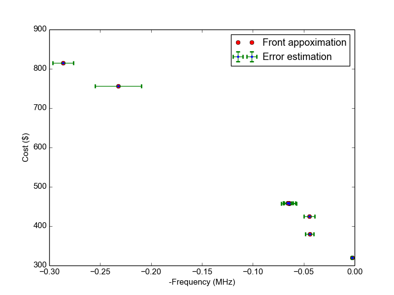
Finally, after run the results of optimization may be represented as approximation of Pareto frontier with error bars.

To run the example, open a command prompt and execute:

python -m da.p7core.examples.gtopt.example_gtopt_mcmisbrdo

You can also get the full code and run the example as a script: example_gtopt_robust_sbo.py.

12.2.6. Intermediate result

This example shows how to obtain intermediate optimization result using a watcher. It considers solving a bi-objective problem and draws a Pareto frontier approximation evolution.

First, some modules for GTOpt functionality, problem definition and miscellaneous things have to be imported:

from da.p7core import gtopt # is required for GTOpt functionality
import matplotlib.pyplot as plt # to show some plots
from math import exp # for objective computation

Second, we define the optimization problem:

class faf(gtopt.ProblemUnconstrained):
  """
  Fonseca and Fleming function.
  Number of variables: n = 2.
  Number of objectives k = 2.
  Source: C. M. Fonzeca and P. J. Fleming, “An overview of evolutionary algorithms in multiobjective optimization,” Evol Comput, vol. 3, no. 1, pp. 1-16, 1995.
  """

#[prepare] begin
  def prepare_problem(self):
    self.n = 2
    for i in range(self.n):
      self.add_variable((-4.0, 4.0))

    self.add_objective(hints={"@GTOpt/EvaluationCostType": "Expensive"})
    self.add_objective(hints={"@GTOpt/EvaluationCostType": "Expensive"})
#[prepare] end
#[objectives] begin
  def define_objectives(self, x):
    n_sqrt = self.n**-.5
    return [- exp(-sum([(t - n_sqrt)**2 for t in x])),
            - exp(-sum([(t + n_sqrt)**2 for t in x]))]
#[objectives] end

In prepare_problem() we setup two-dimensional Fonseca and Fleming function:

  def prepare_problem(self):
    self.n = 2
    for i in range(self.n):
      self.add_variable((-4.0, 4.0))

    self.add_objective(hints={"@GTOpt/EvaluationCostType": "Expensive"})
    self.add_objective(hints={"@GTOpt/EvaluationCostType": "Expensive"})

with objectives defined in define_objectives() implementation:

  def define_objectives(self, x):
    n_sqrt = self.n**-.5
    return [- exp(-sum([(t - n_sqrt)**2 for t in x])),
            - exp(-sum([(t + n_sqrt)**2 for t in x]))]

Third, we define a custom watcher (see description in section Watchers). It can be any Python object implementing the __call__() method with an additional argument:

class IntermediateResult():
  def __init__(self):
      self.counter = 0;

#[callback] begin
  def __call__(self, report):
  #[query] begin
    if report["ResultUpdated"]: # test if there updates for intermediate result are available
      result = report["RequestIntermediateResult"]() #query intermediate result
  #[query] end
      data = plt.plot(result.optimal.f[:, 0], result.optimal.f[:, 1], ".", label="Update %d" % self.counter)
      print("Optimal set size: %s" % result.optimal)
      self.counter += 1
      plt.legend(loc="lower left")
      plt.pause(0.0001) # show results
      data[0].set_label(None)
    return True
#[callback] end

Our watcher always returns True because we are not going to interrupt optimization. We examine msg that is sent to __call__() by Solver.

    if report["ResultUpdated"]: # test if there updates for intermediate result are available
      result = report["RequestIntermediateResult"]() #query intermediate result

The msg in this case is a dictionary with the following information:

• msg["ResultUpdated"] tells whether there are any updates in the intermediate result since the last result query. If it is False, there is no new information available. If True, you can request new optimization results.
• msg["RequestIntermediateResult"] is a callable that actually queries an intermediate result. When called, it returns a Result object.

To set the custom watcher we call Solver.set_watcher() before optimization:

  optimizer = gtopt.Solver()
  optimizer.set_watcher(IntermediateResult())
  result = optimizer.solve(faf(), options={"GTopt/MaximumExpensiveIterations": 200})

You can also get the full code and run the example as a script: example_gtopt_intermediate_result.

12.2.7. Fitting problem

Here we provide an example that shows how to use GTOpt special ProblemFitting class to formulate and solve a fitting problem. The goal is to find parameters of the given model that minimize the distance between the model and given data, i.e.

\[\left(\sum_{i=1}^N \left(f(model_x^i, x) - model_y^i\right)^2/N\right)^{1/2}\]

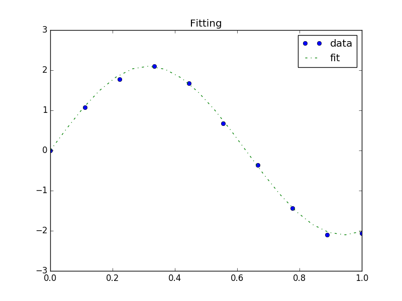
For this example, disturbed image of \(sin\) function is used as original data that is needed to be fit.

def generate_data(N=10):
  task = SineFit([1], [1]) #formally create instance of SineFit to reuse define_models method
  x = numpy.linspace(0, 1, N)
  numpy.random.seed(1234) # fix seed
  y = task.define_models(x, [2, 5]) * (1 +  numpy.random.uniform(-.1, +.1, N))
  return x, y

To formulate a problem ProblemFitting class is defined

class SineFit(gtopt.ProblemFitting):
  def __init__(self, model_x, model_y):
    self.model_x = model_x
    self.model_y = model_y

  def prepare_problem(self):
#[x_sample] begin
    self.add_model_x(self.model_x)
#[x_sample] end
#[variables] begin
    self.add_variable((None, None), 1)
    self.add_variable((None, None), 2)
#[variables] end
#[y_sample] begin
    self.add_model_y(self.model_y)
#[y_sample] end
#[model] begin
  def define_models(self, x, p):
    return p[0] * numpy.sin(p[1] * x)
#[model] end

in which we setup input data \(model_x\)

    self.add_model_x(self.model_x)

parameters of the model

    self.add_variable((None, None), 1)
    self.add_variable((None, None), 2)

the observed output \(model_y\)

    self.add_model_y(self.model_y)

and define the model that should be fit

  def define_models(self, x, p):
    return p[0] * numpy.sin(p[1] * x)

Finally, to fit the model to the given data, the instance of the problem is passed to the instance of the optimizer.

  optimizer = gtopt.Solver()
  task = SineFit(model_x, model_y)
  result = optimizer.solve(task)

The result looks like

To run the example, open a command prompt and execute:

python -m da.p7core.examples.gtopt.example_gtopt_fitting

More GTOpt examples can also be found in Code Samples.