3.7. Robust Optimization
Sections
3.7.1. Overview
Robust single- and multi-objective constrained optimization in GTOpt supports virtually all possible robust formulations, including probabilistic and quantile type constraints. It is based on the original state-of-the-art stochastic approach developed by PSEVEN. The heart of the method is careful adjustment of current number of sampled uncertain parameters: away from optimality it is more than enough to consider only a small number of random realizations, but their number must increase once optimal solution is approached. Moreover, the unique feature of this family of algorithms is that they not only provide the solution itself, corresponding uncertainty estimates of objective and constraint values at found solution are provided as well. A particular advantage of our robust optimization algorithms for engineering applications is that the tool never need to know explicit distribution law of the uncertain parameters, it is enough to provide their distribution only empirically. Moreover, surrogate modeling approaches apply directly within our strategy.
The need to consider robust optimization tasks appears immediately once one realizes that some external to original formulation parameters are not well known in fact. It is crucial that uncertain model parameters make the whole optimization problem not well defined. Indeed, if we ever admit “random” dependencies of problem data (objectives, constraints) then the problem “solution” becomes also random and hence devoid of meaning. One must exclude randomness from the problem and it is common to consider various expectations and moments of relevant distribution. Respectively reformulated optimization task is known as robust counterpart of the original problem and it is by no means unique. Worst-case scenarios are known to be too restrictive and GTOpt does not consider them. Instead, randomness is assumed to be eliminated by taking appropriate expectation values.
Unfortunately, none of these expectations could actually be calculated, we could ever hope to only approximate them. Then an immediate prime problem is how tight the approximation must be. Indeed, one would like to consider rough but cheap approximations, but simultaneously one must provide high enough accuracy to properly represent hypothetical original “true” problem, in which expectation are calculated exactly (in what follows the term “original” refers to such hypothetical “exact” formulation). As it usually happens, the optimal strategy turns out to be adaptive: the closer optimal solution is the tighter our approximations must be.
Side effect of our inability to explicitly consider original problem is that we could only obtain approximate (candidate) solutions. Then it is not surprising that every candidate solution must be validated to ensure its closeness to the solution of original problem. Note that this is an example of robust optimization specific features, not present in usual non-robust cases.
Here significant difference between computationally cheap and expensive problems arises. Indeed, validation of solution candidates might be performed automatically only in former case. For expensive problems verification of even a single design might be too costly and hence requires explicit end-user (decision maker) intervention. This is the policy accepted by GTOpt in Robust Design Optimization (RDO) algorithms: once even a single expensive to evaluate observable (objective or constraint) is found in input problem GTOpt refuses to automatically verify proposed solution set. Instead, total set of solution candidates is presented to end-user together with available statistical estimates of respective performances and constraints, which are required to perform proper design selection.
Another difficult to treat issue within the RDO framework is the appearance of new type of constraints, so called chance constraints. They are hard to consider because even moderate accuracy evaluation of them is extremely expensive, while corresponding naive approximations lead to strongly discontinuous subproblems. Proposed remedy is to construct smooth over-estimators of chance constraints such that the corresponding accuracy increases as algorithm proceeds.
3.7.2. Quantitative Discussion
It should be noted that general discussion presented in this section mainly concerns computationally expensive problems. Application of the ideas, outlined here, in expensive context has almost no practical significance (although they are perfectly applicable theoretically). Issues specific to computationally expensive case are presented in the next section.
3.7.2.1. Robust Problem Formulation
In majority of practical applications “classical” formulation of optimization problem
is not adequate. In reality, problem data \(f, c\) additionally depend upon external “random” parameters \(\xi\) from some uncertainty set \(U_\xi\):
In this circumstances optimal solution \(x^*\) becomes also dependent upon “random” realizations of \(\xi\)
and hence is devoid of meaning. Therefore, already at the level of problem formulation we must consider dependence upon external parameters
Evidently, one should get rid of \(\xi\)-dependence of the solution
Decision on what is the optimal solution \(x^*\) must be taken “here and now”, before concrete realization of \(\xi\) is known! Depending on concrete meaning of the reduction \(x^*(\xi) \to x^*\) various formulation of robust optimization problems are possible. For instance, if we know probability distribution \(\rho(\xi)\) of uncertain parameters we could consider
Constraints are more tricky, there are several possibilities:
- Expectation constraints: \(\vec{c}_L \,\le\, \vec{E}[ c(x,\xi) ] \,\le \, \vec{c}_U\).
- Chance constraints: \(P\{c^i_L \,\le\, c^i(x,\xi) \,\le \, c^i_U \} \ge 1 - \alpha \quad \alpha \in (0:1)\).
GTOpt handles following robust optimization problem:
3.7.2.2. Approximated Problem
GTOpt adopts stochastic approximation to the averages considered in the problem statement. Advantages of stochastic approach:
- Details and concrete form of probability densities \(\rho(\xi)\) are completely delegated to end-user.
Note that in real-life applications determination of appropriate \(\rho(\xi)\) might be very difficult.
- It is enough to know only empirical distribution \(\rho(\xi)\) without any analytical equations.
- Uncertainty set \(U_\xi\) is never used explicitly.
- “Universality”: stochastic formulation is suitable for virtually all cases.
However, there are a few notable disadvantages as well:
- Effective solution of stochastic optimization problems requires specific approaches!
Prime difficulty here is that none of expectations \(E[...]\) or probabilities \(P\{...\}\) could ever be calculated exactly. But then the question is: what is the meaning of sole “solution” of stochastic problem? The point that it is not enough to simply “solve” approximated problem. One must ensure that found approximate solution is indeed “almost” optimal and “close” to the solution of original problem. Therefore, the prime difficulty in solving stochastic task reduces to the fact, that we not simply want to find the solution, we must also validate proposed candidate.
As far as utilized in GTOpt stochastic approximation is concerned, the underlying idea is simple:
where \(\{\xi_i\}\), \(i = 1,...,N\) is finite \(\xi\)-sample given externally and presumably distributed with \(\rho(\xi)\).
Prime questions to be discussed:
Since sample size \(N\) is always finite — what might be “the answer” for the original problem?
How large \(N\) must be taken? How it depends upon optimality of current approximate solution?
What should we do with chance constraints since at finite \(N\) straightforward approximation
\[P\{g(x,\xi) \ge 0\} ~ \approx ~ \frac{1}{N} \sum\nolimits_i \Theta( g(x,\xi_i) ) \equiv p_N(x)\]is discontinuous (discontinuities being of order \(\sim 1/N\)).
3.7.2.3. Approximated Problem Solution
Concerning the meaning of approximated with finite sample solution we note that for any solution \(x\) of arbitrary optimization problem it is natural to consider two characteristics:
Feasibility measure \(\psi(x)\) (see section Optimal Solution for details).
Optimality measure \(\theta(x)\):
\[\theta(x) = \min\limits_{\lambda_i \ge 0} \left| \nabla f(x) ~+~ \sum_i \lambda_i \, \nabla c^i(x) \right|^2\]which is nothing but the norm of KKT conditions residual.
In stochastic context we should also consider corresponding stochastic approximations \(\psi_N\), \(\theta_N\). Therefore, the most complete answer available in stochastic approach reduces to:
Probability that feasibility measure of approximate solution \(x^*_N\) is greater than given tolerance \(\delta\psi\) is less than predefined threshold Y%
\[P\{ \, \psi(x^*_N) > \delta\psi \,\} \le Y\%\]Probability that optimality measure of approximate solution \(N\) is greater than given tolerance \(\delta\theta\) is less than predefined threshold X%
Parameters \(\delta\psi\) and \(\delta\theta\) are to be given externally. Quantiles Y% and X% might be taken constant (commonly accepted value is 5%).
Now we could summarize generic scheme to solve stochastic optimization problem:
- For sufficiently large sample size \(N\) approximate original problem.
- Solve approximated task to obtain candidate solution \(x^*_N\) with usual means.
- Question: since solution of approximated subproblem is also approximate — what are the appropriate tolerances \(\epsilon^\psi_N\), \(\epsilon^\theta_N\) to be used in finding candidate \(x^*_N\)?
- Check statistics of obtained candidate: ensure that both expectations \((\theta_N, \psi_N)\) and statistical uncertainties \((\delta\theta_N, \delta\psi_N)\) are sufficiently small.
- If statistical precision of candidate is insufficient, enlarge sample size and continue with next cycle.
3.7.2.4. Efficient Sample Size Selection
Thus the central question to the whole approach is how to select current sample size efficiently. To address it let us note that at every stage of stochastic problem solution there are two different sources of uncertainties: statistical uncertainties, \(\sim 1/\sqrt{N}\), and “systematic” uncertainties (tolerances of optimization at every fixed \(N\)). As it usually happens, optimal strategy is to keep both statistical and systematic errors of the same order. This simple observation allows to unambiguously fix required tolerances \(\epsilon^\psi_N\), \(\epsilon^\theta_N\) to obtain candidate solution and current sample size. Thus we could summarize the scheme of efficient algorithm to solve stochastic problem:
Set initial (relatively small) sample size \(N\) [heuristics] and \(\mu=0\).
Consider the statistics at initial point \(x^*_{N,\mu}\):
- Calculate statistical uncertainties \((\delta\theta_{N,\mu}\), \(\delta\psi_{N,\mu})\).
- Set the tolerances \(\epsilon^\psi_{N,\mu} \sim \delta\psi_{N,\mu}\), \(\epsilon^\theta_{N,\mu} \sim \delta\theta_{N,\mu}\) for optimization at the initial stage.
Optimization of \(N\)-approximated problem with tolerances \((\epsilon^\psi_{N,\mu}\), \(\epsilon^\theta_{N,\mu})\), obtaining the next candidate solution \(x^*_{N,\mu}\).
Validation of candidate solution \(x^*_{N,\mu}\): statistics estimate in \(x^*_{N,\mu}\), evaluation of \((\delta\theta_{N,\mu}\), \(\delta\psi_{N,\mu})\). Finished if statistics is good enough.
Estimation of required sample size \(N_{next}\) for the next iterate:
\[N_{next} ~=~ N \,\,\cdot\,\, \mbox{heuristics}\{\,\, (\frac{\delta\theta_N}{\delta\theta})^2 \,\, , \,\, (\frac{\delta\psi_N}{\delta\psi})^2 \,\, , \,\, x^*_{\mu-1}, x^*_{N,\mu} \,\,\}\]- \(\delta\theta\), \(\delta\psi\) are the required precisions.
- Heuristics keeps \(N_{next}\) in reasonable limits, depends upon the made progress.
Rescaling of optimization tolerances with factor \(\sim \sqrt{N/N_{next}}\) which expresses “statistics” \(\approx\) “systematics”.
New iteration (3) for \(N\)-approximated problem with \(N = N_{next}\).
3.7.2.5. Chance Constraints Treatment
Now it is time to discuss efficient treatment of chance constraints. Idea is to consider continuous majorant of the original discontinuous stochastic approximations tightening approximation with increasing \(N\). In equations:
where \(\Theta(x)\) is a step function, \(R_\varepsilon(x)\) is a (smooth) majorant of \(\Theta(x)\) and \(\varepsilon = \varepsilon(N)\):
Notable issue, which we could only mention here (it is successfully resolved in GTOpt), concerns apparent conformal (scale) non-invariance of proposed approach:
The point is that regularization revives former zero mode and this have taken into account. Solution is to dynamically adjust the scale parameter:
or even better (to avoid singularity at \(t=0\)):
Another issue arises when regularized problem appears to be infeasible. One can see that from \(E[R_\varepsilon(g)] > \alpha\) it does not follow that \(E[\Theta(g)] > \alpha\) for any positive \(\varepsilon\). Hence decision on infeasibility of original problem must be delayed until regularization is completely removed.
3.7.2.6. Robust Problem Optimal Solution
Above (see Optimal Solution) we have defined the optimal set for classical optimization problems. For robust optimization we have to refine the formulation. The main difference is that due to the approximative approach (see Approximated Problem) objectives (and constraints) are known with a certain (stochastic) error. Therefore we cannot directly compare their averages. Instead, GTOpt uses interval arithmetics to detect optimality of designs that turns even a single objective problem into somewhat multiobjective.
We start from unconstrained case. Let \(x^1\) and \(x^2\) be two points from which we should select the best. Let \(\tilde{f}(x^1)\) and \(\tilde{f}(x^2)\) be the estimated averages of objectives for these points. These estimates themselves can be considered random realizations, so the average of an estimate is the same as the average of randomized objective realizations. But what we are interested in is whether they are stable, that is, the standard deviation of these average estimators. Using the sample-based approach the estimators \(\delta\tilde{f}(x^1)\) and \(\delta\tilde{f}(x^2)\) for standard deviation of averages’ estimators can be constructed (see section below).
If
then \(x^1\) is better. Vice versa, if
then \(x^2\) is better. Otherwise accuracy is not enough to take a decision. In the last case GTOpt either improves statistics (if it may increase a sample) or returns both points, considering them incomparable.
To take a decision about optimality in constrained case we at first must determine if the point is feasible. Let \(\tilde{\psi}(x^1)\) be the estimator of the average feasibility measure (see section Optimal Solution for details), and \(\delta\tilde{\psi}(x^1)\) be its estimated error. GTOpt consider the point feasible if \(\tilde{\psi}(x^1) - \delta\tilde{\psi}(x^1) \le 0\).
Thus
if GTOpt/OptimalSetType is "Strict"
results include points that are feasible and incomparable in interval sense.
Note that GTOpt does not seek (or approximate) all such points,
the goal is to
approximate the true optimal solution of the problem (when all statistical values are evaluated precisely),
however it
keeps almost all points (those that are too close are filtered out, set by GTOpt/OptimalSetRigor)
incomparable points met along the infinity way to true optimal solution.
If GTOpt/OptimalSetType is set to "Extended",
\(\tilde{\psi}\) is considered an additional special objective.
The point \(x^1\) has better feasibility measure than the point \(x^2\) if
The results that are non-dominated (in space \(f\) and \(\psi\)) and feasible go to optimal set and non-dominated infeasible results go to infeasible set. Note that such definitions of optimality and feasibility imply that a point that is feasible with its error cannot be dominated by a point that has feasible average but its error violates constraints, however both points are considered feasible.
3.7.2.7. Notes on Statistics Estimation
Efficiency of the whole approach to robust optimization crucially depends upon our ability to perform statistics estimation in most economical way. Indeed, it potentially requires a lot of additional model evaluations without any progress in design variables. Let us note that one of the standard approaches considers auxiliary additionally generated ensemble \(\{x^*_N\}_i\), \(i = 1, .., M\), which is extremely expensive (requires \(\sim (M - 1) \cdot N \,\gg\, N\) additional evaluations). Solution implemented in GTOpt is to use fairly well known jackknife method, which does not require additional evaluations at all.
3.7.2.8. Mean Variance Optimization
Particular but common case of robust bi-objective optimization is minimization both expectation and variance of the same observable.
Technically, with auxiliary variables and constraints this problem can be reduced to a bi-objective form with only minimized expectations. But such reformulation loses a property that different entities are constructed from the same function. So GTOpt has embedded support for the mean-variance problem in the original form in which the user has to provide only one function.
Despite the only function is used the solution is set of points approximating Pareto front in space of two objective: mean and variance.
3.7.2.9. Illustrative Examples
Quantile optimization example taken from Theory and Practice of Uncertain Programming, B. Lu, 2009.
\[ \begin{align}\begin{aligned}\begin{array}{c}\\\begin{split}\begin{array}{c} \min \,\, \phi \\ \end{array}\end{split}\\\begin{split}\begin{array}{l} c_1 \equiv P\{\,\, 0 \,\le\, \sum\nolimits_{i=1}^3 \,\zeta_i \, x_i ~+~ \phi \,\,\} \,\ge\, 0.9 \\ c_2 \equiv P\{\,\, \sum\nolimits_{i=1}^3 \,\eta_i \, x^2_i \,\le\, 8 \,\,\} \,\ge\, 0.8 \\ c_3 \equiv P\{\,\, \sum\nolimits_{i=1}^3 \,\tau_i \, x^3_i \,\le\, 15 \,\,\} \,\ge\, 0.85 \end{array}\end{split}\\\begin{split}\begin{array}{c} \zeta_1 \sim U(1,2) \qquad \eta_1 \sim U(2,3) \qquad \tau_1 \sim U(3,4) \\ \zeta_2 \sim N(1,1) \qquad \eta_2 \sim N(2,1) \qquad \tau_2 \sim N(3,1) \\ \zeta_3 \sim Exp(1) \qquad \eta_3 \sim Exp(2) \qquad \tau_3 \sim Exp(3) \end{array}\end{split}\\\end{array}\end{aligned}\end{align} \]
- \(U(a,b)\): uniform distribution on \([a;b]\).
- \(N(a,b)\): normal distribution with mean \(a\) and variance \(b\).
- \(Exp(a)\): exponential distribution with parameter \(a\).
In cited above reference genetic algorithm with meta-modeling was used, the result is:
\[\begin{split}\begin{array}{c} \underline{1.5 \cdot 10^7 \mbox{evaluations}} \\ x^* \approx (1.404, 0.468, 0.924) \qquad f^* \approx -2.21\\ c_1 \approx 0.9 \quad c_2 \approx 0.8 \quad c_3 \approx 0.85 \end{array}\end{split}\]Note that the meaning of \(\approx\) was not clarified. Application of our approach with required tolerances \(\delta\theta, \delta\psi = 2.5\%\) gives:
\[\begin{split}\begin{array}{c} x^* = (1.53, 0.44, 0.61) \qquad f^* = -2.22(3) \\ c_1 = 0.92(2) \quad c_2 = 0.85(2) \quad c_3 = 0.88(2) \end{array}\end{split}\]with only \(\approx 4.2 \cdot 10^4\) evaluations, which is by 3 orders of magnitude smaller than the number cited above.
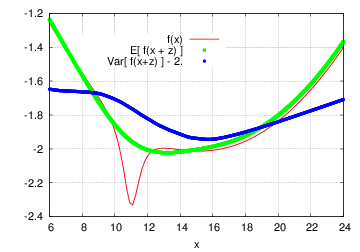
Robust bi-objective optimization (mean-variance optimization).
Let \(f(x) = - \frac{1}{5 (11 - x)^2 + 2} + \frac{1}{120}\, (x - 15) (x - 16) - 2\). Then the problem is:
\[\begin{split}\begin{array}{c} \min\,\,( \,\, E[\, f(x+\xi)\,]\,\, , \,\, Var[\,f(x + \xi)\,] \,\,) \\ x \in [0:28] \quad \xi \sim N(0,2) \end{array}\end{split}\]Pareto set is known to be located in \(x \in [13.2 ; 15.75 ]\).
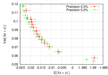
Depending on externally given tolerances GTOpt robust optimization algorithms require
\[\delta\theta = 0.3\% : 6\cdot 10^5 \qquad \delta\theta = 0.2\% : 1.1\cdot 10^6\]evaluations, which have to be compared with typical evaluation count of Monte-Carlo based methods, \((5 \div 8) \cdot 10^6\).
3.7.3. Notes on Surrogate Based Robust Optimization
Surrogate-based (SBO) methodology is widely believed to be efficient approach to handle computationally expensive problems. It is natural then to apply SBO strategy in RDO context as well, however, there are a few notable issues which make SBO RDO algorithms quite distinct. First, we cannot afford to consider even a moderate number of replications (sample sizes) for all proposed designs, sample size selection must be twice careful in expensive context. Second, for relatively small number of replications statistical uncertainties of respective estimates cannot be ignored in SBO-driven optimization: already at the level of surrogate models construction as well as during the optimization of SBO-specific criterion uncertainties play significant role. This requires, in particular, to change SBO methodology itself:
- We should explicitly allow non-interpolating models, which deviate from predicted data points by the amount, derived from currently available statistics.
- SBO-specific criterion is to be changed. For instance, the very notion of best attained so far solution becomes illusive when uncertainties are large.
- Selection of the best designs becomes highly non-trivial. Moreover, budget allocation within each SBO iteration requires to solve rather complicated internal subproblem.
In all other respects qualitative scheme of SBO RDO strategy does not change significantly compared to what had been discussed previously. Namely, GTOpt starts with some small number of replications allocated to each potential design and runs a first iteration of SBO. Then for all so far accumulated designs internal Optimal Computation Budget Allocation (OCBA) problem is solved, its outcome allows to determine designs, which are worth to be additionally sampled. After resampling of (hopefully) small fraction of designs next SBO round takes place.
Important feature of the above strategy is that GTOpt never tries to validate proposed set of optimal designs. As was already mentioned, automatic verification of candidate solutions is too risky for expensive problem and is to be delegated to end-user (decision maker). To facilitate this, GTOpt provides end-user with all available information on estimated optimal set including achieved so far statistical uncertainties.
3.7.4. Using Stochastic Variables
The distribution argument in set_stochastic()
is an object of your custom class which implements the probability distribution.
The stochastic distribution should be set in the prepare_problem()
method of the problem’s class, for example:
class StochasticProblem(gtopt.ProblemUnconstrained):

    # other definitions

    def prepare_problem(self):

        # other problem properties

        self.set_stochastic(MyDistribution(*args))
The distribution class which you implement must provide the
getNumericalSample() and
getDimension() methods.
-
Distribution.getNumericalSample(quantity)¶ Get values from the distribution.
Parameters: quantity ( int) – the number of distribution realizationsReturns: generated values Return type: array-like, 1D This method should return a list or some 1D array, which length is quantity multiplied by the distribution dimension. Value generation is up to you: for example, you can do it dynamically or get values from a pre-generated pool.
-
Distribution.getDimension()¶ Get distribution dimension, or the number of stochastic variables in the problem.
Returns: distribution dimension Return type: intMultiple stochastic variables are added to a problem by creating a multidimensional distribution. Since
getNumericalSample()returns all values as an 1D array, GTOpt needs this method to get the dimension of a single variable vector.
See also
- example_gtopt.py code sample
- Basic GTOpt example including a robust optimization problem.
- example_gtopt_rdo.py code sample
- General robust optimization example.
- Surrogate Based Robust Optimization example
- Advanced robust optimization example.