3.4. Noisy Problems

3.4.1. Noisy vs Meaningless Problems

In practical applications optimization data is often “noisy”. Qualitatively this means that

\[\mbox{"}\,\,\forall x_0 : \,\,\quad \lim_{x\to x_0} f(x) \ne f(x_0)\,\,\mbox{"}\]

Despite of symbolic meaning, this formula signifies two vastly different modes:

• Small relative noise: \(|f(x_0) - f(x)| \ll |f(x_0)|\)

  

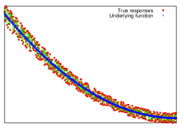
• Large relative noise: \(|f(x_0) - f(x)| \gtrsim |f(x_0)|\)

  

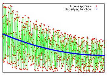
Key difference between these two cases is the separation of scales (or its absence for meaningless problem):

\[\exists L \, : \quad \frac{|f(x) - f(y)|}{|f(x) + f(y)|} \gtrsim 1 \qquad \forall x,y \,: \,\, |x-y| \gtrsim L\]

Therefore, model is considered “noisy” only if scales separation could be established. Otherwise, given model should not be optimized (the answer makes no sense anyway).

3.4.2. Accepted Noise Model

GTOpt accepts the following model of noisy data. Actually measured response is assumed to have generic form:

\[f(x) = f_0(x) \cdot (1 + \epsilon_x) \qquad \epsilon_x \ll 1\]

It is seen trivially that conventional gradient-based methods have serious difficulties upon considering noisy data:

\[\partial f = \partial f_0 \cdot (1 + \epsilon_x) + f_0 \cdot \partial \epsilon_x \qquad |\epsilon_x| = +\infty\]

It is commonly accepted that derivative-free optimization (DFO) is the only approach in noisy context!

Note, however, that majority of implemented methods are gradient-based. Could we redefine the very notion of “gradient” to make it suitable for noisy data?

3.4.3. Framed Gradients

3.4.3.1. General Ideas

Consider the standard finite difference scheme

\[\begin{split}\begin{array}{c} f(x + \Delta x) \sim f(x) + f_0 \cdot \epsilon + f'_0 \cdot \Delta x + O(\Delta x^2) \\ \epsilon ~\sim~ |\epsilon_x| ~\sim~ |\epsilon_{x + \Delta x}| ~\sim ~ |\epsilon_x ~-~ \epsilon_{x + \Delta x}| \end{array}\end{split}\]

where the last line follows from the assumed noise model. Nearby figure illustrated how the error of above approximation changes if we vary \(\Delta x\). Evidently, for any given reasonable \(\epsilon_x\) there exists “optimal” \(\Delta x\) such that approximation error is minimized. Note by the way how minimal value of approximation error ceases to exist once scales separation becomes impossible.

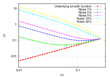
Approximation error for the above scheme

\[|\Delta f'| \sim ~ \frac{\epsilon}{\Delta x} ~+~ \mathrm{const} \cdot \Delta x\]

is minimal at \(\Delta x_{opt} ~ \sim ~ \sqrt{\epsilon}\). Unfortunately, the noise factor \(\epsilon\) cannot be guessed a priori! In any case, one concludes that fixed step sizes are inappropriate:

• At small \(\Delta x\) we are essentially differentiating the noise.
• Large \(\Delta x\) cannot ensure convergence for obvious reasons.

Ideally, we should consider adaptive step size selection:

• Away from optimal solution \(\Delta x\) is allowed to be relatively large.
• Close to optimality \(\Delta x\) must diminish to ensure convergence.

Thus, we are going to consider current step size as a function of distance to optimal solution:

\[\Delta x ~=~ \Delta x(\, |x ~-~ x^*| \,)\]

Simultaneously, we want to have cheap and “universal” rules for step size selection. Is there any possibility to define appropriate rules universally (algorithm independent)?

Our analysis is based on observation that vast majority of optimization algorithms are iterative, each iteration being generically represented by

\[x_{\mu+1} ~=~ Alg(\,x_\mu\,)\]

If we consider algorithm \(Alg(x)\) as unknown without any means to look into its internals then only the sequence \(\{x_1, x_2, ..., x_\mu,... \}\) is available for consideration. But for any “meaningful” (converging) algorithm \(Alg\) we have

\[|x_{\mu+1} - x_\mu| \equiv |\delta x_\mu| ~\to ~ 0 \qquad \mbox{as} \qquad \mu ~\to ~\infty\]

Thus it is natural to force \(\Delta x\) to depend on iteration count via

\[\Delta x ~\to ~ \Delta x_\mu = \Delta x(|x_{\mu+1} - x_\mu|)\]

Moreover, the simplest dependence is given by linear proportionality \(\Delta x \sim |x_{\mu+1} - x_\mu|\). In practice, some kind of averaging with respect to particular history window is to be performed. Therefore, our ansatz states that currently selected step size is proportional to averaged over recent history algorithm progress:

\[\Delta x_\mu ~ \sim ~ \langle |\delta x|_\nu \rangle \quad \nu = \mu, \mu - 1, ..., \mu - K\]

Prime advantage of the above relation is its adaptiveness:

• When \(Alg\) stalls \(\Delta x_\mu\) rapidly diminishes thus increasing accuracy and allowing algorithm to proceed.
• When \(Alg\) performs well \(\Delta x_\mu\) remains relatively large to allow significant progress even in noisy context.

However, we did not specify yet the initial value of the step size \(\Delta x_0\). Note that within the accepted noise model \(f = f_0 \cdot (1 + \epsilon)\) the need to capture derivatives of \(f_0\) and not of the noise \(\epsilon\) requires that

\[f(x + \Delta x) - f(x) ~ \gg ~ \epsilon \, f_0 ~ \approx ~ \epsilon f\]

which might be translated into the requirement on noise magnitude:

\[\epsilon ~ \ll ~ \frac{f(x + \Delta x) - f(x)}{f(x)}\]

In particular, at very first iteration \(\Delta x\) is to be chosen according to this equation, however, specific noise magnitude is never known. The way out is provided by bounding acceptable noise magnitudes from above:

\[|\epsilon_x| \le \epsilon_0\]

where \(\epsilon_0\) is some predefined externally given parameter (expected noise level), which for well posed noisy problems might be estimated as \(\epsilon_0 \sim 0.1 \div 0.2\). In other words, initial \(\Delta x\) must be chosen such that relative function change is (much) larger than expected noise level.

3.4.3.2. Technical Details

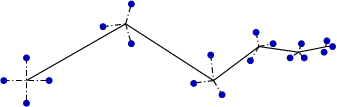
Proper estimation of gradients \(\nabla f\) requires the following data to be provided:

• Full rank framing basis \([\Delta x]_{ir}\), \(i = 1, ..., N\), \(r = 1, ..., R\).

  \[\Delta f_r ~=~ \sum_i [\nabla f]_i \cdot [\Delta x]_{ir} \qquad \mbox{Rank}( \Delta x ) ~=~ N\]

• Framing basis must be sufficiently away from being degenerate.

Simultaneously, we must ensure smallness of estimation error. In general, precision of derivatives estimate might be improved by:

• Squeezing the differentiation scale \(\Delta x \to 0\).
• Switching to higher order approximation schemes.

In current approach \(\Delta x\) is not in our disposal. Thus, the problem is how to adaptively improve approximation scheme and quality?

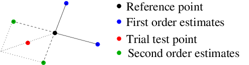
Solution is provided by adaptive first/second order switching policy, which is simple enough be to explained algorithmically:

• Let \(x_0\) be reference point with framing basis \([\Delta x]_{ir}\).
• For \(R = N\) take an additional point \(x_0 - 1/N \sum_r \Delta x_r\) to be included into \([\Delta x]\).
• Let “prime” (least degenerate) vectors \([\Delta x]_{ir}\) are \(v_\alpha\), \(\alpha = 1, ..., N\).

Then:

1. Always start with first order estimates on simplex \(\{ x_0, x_0 \pm v_\alpha\}\).
2. Estimate derivatives with all points included.
3. Stop if two estimates only slightly different.
4. Otherwise, compute second order approximations.

In the considerations above lengths of framing basis vectors were essentially the same:

\[|[\Delta x]_r| ~\approx ~ \mbox{const}\]

This is absolutely inappropriate for badly conditioned problems: \(\Delta x\) components corresponding to directions of large local curvature must be (much) smaller in order to give adequate estimates of corresponding “partial” derivatives. To circumvent this consider again the “random” sequence \(\{\delta x_\mu\}\):

\[\delta x_\mu ~ \equiv ~ x_{\mu+1} - x_\mu \qquad x_{\mu+1} ~=~ Alg(x_\mu)\]

We actually exploited above a particular first moment \(\langle |\delta x| \rangle\) taken with respect to this distribution:

\[\Delta x_\mu ~ \sim ~ \langle|\delta x_\nu|\rangle \quad \nu \le \mu\]

Can we find anything useful in higher order moments? Since the magnitude \(|\delta x_\mu|\) was accounted for already, it is natural to consider

\[\begin{split}\begin{array}{rcl} E &\equiv&\langle \, \delta \hat{x}_\nu \, \delta \hat{x}_\nu^T \, \rangle \qquad \\ \delta \hat{x}_\nu &=&\delta x_\nu / |\delta x_\nu| \end{array}\end{split}\]

which expresses directional correlations of \(\delta x_\mu\) vectors. Our assertion is that the eigensystem \(\{\lambda_i, \vec{e}_i\}\) of \(E\), \(E \cdot e_i ~=~ \lambda_i \,\, e_i\) quantitatively reflects the condition number of underlying problem. Ultimately, this is because:

• \(Alg(x)\) as a convergent algorithm must use something like “sufficient decrease” criteria at each step (well, we slightly squeeze the number of suitable algorithms, the ones based on non-monotonic line search are not appropriate. However, absolute majority of methods do utilize sufficient decrease criteria).

Therefore, in first approximation the recipe to account for local curvature might look like:

• Monitor not only current framing basis scale \(\langle |\Delta x_\mu |\rangle\), but also directional cross-correlations:

\[\langle \, \delta \hat{x}_\nu \, \delta \hat{x}_\nu^T \, \rangle \quad \to \quad \{\lambda_i, \vec{e}_i\}\]

• Impose asymmetry of order \(\lambda_i / \lambda_{min}\) along \(e_i\) directions on framing basis keeping framing scale constant, \(\langle |\Delta x_\mu |\rangle\).

To illustrate the above idea let us consider well known BrownBS function,

\[f = (x_0 - 10^3)^2 + (x_1 - 2\cdot 10^{-3})^2 + (x_0 x_1 - 2)^2\]

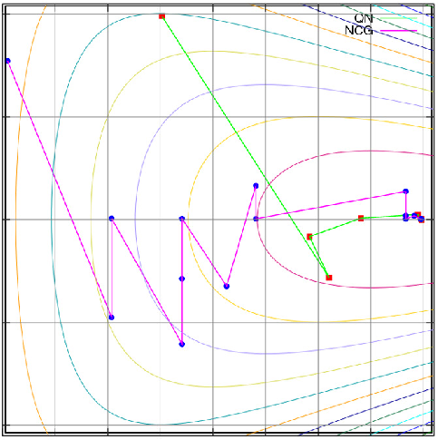
Note huge hierarchy of scales:

• vertical scale: 1
• horizontal scale: 1000

Local condition number near the optimal solution is about \(\chi \approx 10^6\). Application of above approach gives \(\lambda_{max} / \lambda_{min} ~\approx ~ 10^6\) which is totally consistent with analytically known \(\chi\).

3.4.4. Summary

1. Possible noise in problem data is accounted for at the lowest level of GTOpt stack. In particular, noise treatment is completely unrelated to details of concrete optimization algorithms.
2. The essence of our approach is to redefine the notion of all derivatives: for noisy data they are to be understood as finite differences with adaptive step size taken in locally varying basis.
3. Step size is defined by the current progress of upper-level optimization algorithm. In particular, it automatically adjusts itself during the optimization process.
4. Our approach (framed derivatives) allows majority of conventional gradient-based methods to remain operational with essentially no modifications.
5. Framing basis is automatically adjusted not only to current algorithm progress, but also to local condition number of underlying problem. In particular, method works flawlessly even with noisy ill-conditioned tasks.