7.2. Techniques

7.2.1. Space-Filling DoE techniques

Space-filling techniques in GTDoE are aimed to generate uniform samples in the hypercube, possibly in high dimensions. The exact meaning of “uniformity” depends on the application. There are several strategies for defining uniformly distributed point sets.

• Producing point sets whose projections onto lower-dimensional faces of the hypercube are themselves well distributed. Discrepancy measures are usually used to evaluate the quality of such point sets.
• Producing point sets that are well-distributed volumetrically in the hypercube.

Space-filling GTDoE techniques support all types of variables, except the low-discrepancy sequence techniques (Sobol, Halton, Faure), which support only continuous variables. For full details, see section Types of Variables.

7.2.1.1. Random Sampling

Random sampling represents the simplest, yet often useful approach — uniform generation of random points in a hypercube.

• Pros
  • Universality and flexibility
  • Can always be extended by more points
• Cons
  • Low uniformity, especially in high dimensions

Configuration

Random Sampling technique has no options. To use this technique to generate DoE set GTDoE/Technique to RandomSeq.

Figure: Example of space-filling with Random sampling

7.2.1.2. Latin Hypercube Sampling

Latin hypercube sampling (LHS) is a popular and effective technique based on preservation of uniformity of marginal distributions. It’s done by dividing the range of each design variable into \(N\) equal intervals and putting one point in each. So, in the context of statistical sampling, a multidimensional grid containing sample positions is a Latin hypercube if (and only if) there is only one sample in each such interval. \(N\) sample points are placed to satisfy the Latin hypercube requirements. This forces the number of intervals, \(N\), to be the same for each variable. Also note that LH sampling scheme does not require more samples for more dimensions (factors); this independence is one of the main advantages of this sampling scheme.

It should be noted that because of random shuffling, there is a probability that resulting DoE may fill design space very unevenly. However, this probability rapidly declines with the growth of \(N\).

Figure: Latin Hypercube explanation

• Pros
  • Good low-dimensional projection properties
  • Very fast generation
  • Supports categorical variables
• Cons
  • Non-zero probability to generate non-uniform design set
  • Almost impossible to complement/reduce design set without breaking LH properties

Configuration

LHS technique has no options. Set GTDoE/Technique to LHS to use the technique.

Figure: Example of space-filling with LHS sampling

7.2.1.3. Optimized LHS

Optimized LHS (OLHS) is an improved version of LHS. As it was mentioned, plain LH generation may sometimes produce undesirable result. To avoid this, optimization of space-filling criteria can be used (see Uniformity in Definitions). This significantly increases design set generation time and probability of generating required robust DoE.

Figure: This design set perfectly fits LH definition, however lack of space-filling is obvious

Figure: Optimized Latin Hypercube

• Pros
  • Good low-dimensional projection properties
  • High reliability
  • Supports categorical variables
• Cons
  • OLHS is about one hundred times slower than simple LHS
  • Almost impossible to complement/reduce design set without breaking LH properties

Configuration

The user can control the number of optimization iterations by setting GTDoE/OLHS/Iterations option. Larger number of iterations improves uniformity of the resulting sample, but increases generation time.

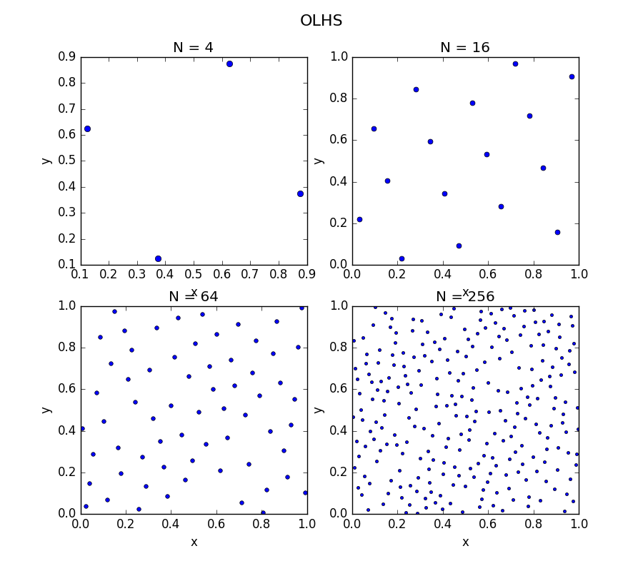
Figure: Example of space-filling with OLHS sampling

7.2.1.4. Full Factorial

Full Factorial technique is a very straightforward approach to generating designs: take all possible combinations of design variables.

To build a Full Factorial design for continuous variables, we need to select some set of \(l\) discrete levels. It is done by uniformly partitioning each parameter range. Thus, for \(d\) continuous variables with \(l\) levels each we get \(l^{d}\) points in design grid, so the approach rapidly becomes computationally infeasible.

This technique also supports discrete and categorical variables (see Types of Variables). A Full Factorial design for discrete (categorical) variables includes all possible combinations of levels (categories). If all variables are discrete (categorical), the design includes exactly \(\prod_{k \in K} i_k\) points, where \(K\) is the number of variables and \(\{i_k\}_{k = 1}^{K}\) is the number of levels (categories) for the k-th variable. If there are \(d\) total variables, where \(K \lt d\) are discrete (categorical) and \(d-K\) are continuous, the number of design points is equal to \(l^{d-K} \cdot \prod_{k \in K} i_k\).

Please note that the technique may generate less points than the requested number \(N\):

• For a design including continuous variables only: if \(N\) can not be represented as \(l^{d}\), only \({\lfloor N^{\frac{1}{d}} \rfloor}^{d}\) points are generated.
• For a design with \(d\) variables total, \(K\) of them being categorical: if \(\frac{N}{\prod_{k \in K} i_k}\) can not be represented as \(l^{d}\), only \({\left \lfloor \left(\frac{N}{\prod_{k \in K} i_k}\right)^{\frac{1}{d}} \right\rfloor}^{d}\) points are generated.

• Pros
  • Low value of uniformity metrics
  • Very fast generation
• Cons
  • Can be built only for a fixed number of points
  • The number of points required for a Full Factorial design grows very fast with increasing design space dimensionality \(d\) and/or the number of levels \(l\), so it becomes infeasible in high-dimensional spaces for any reasonable \(l\)

Configuration

Full Factorial technique has no options. Set GTDoE/Technique to FullFactorial to use the technique.

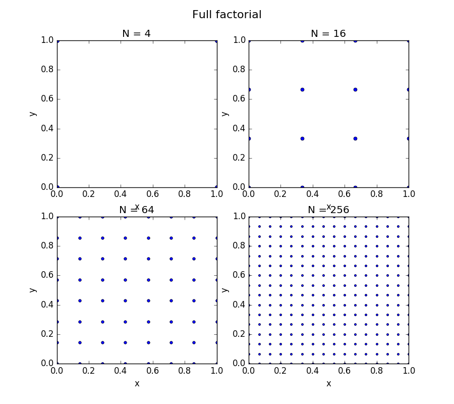
Figure: Example of space-filling with OLHS sampling

7.2.1.5. Fractional Factorial

Fractional factorial design is a DoE consisting of a subset of a full factorial design. It is based on the suggestion that the behavior of a response is dominated by main effects and low-order interactions (see also Sobol indices). This allows to expose information about the most important design variables while using a small fraction of a large full factorial design.

The generation process is based on a structure that determines main factors and interactions between factors. A common way to describe such structure is to use the so-called Generating Strings.

• Pros
  • Fast generation
  • Supports categorical variables
  • Allows to separate main effects and low-level interactions from one another.
• Cons
  • DoE may be highly non-uniform.
  • Categorical variables must have only 2 levels.

Configuration

Generating string for Fractional Factorial DoE can be set by GTDoE/FractionalFactorial/GeneratingString option.

This option uses the conventional fractional factorial notation to create an alias structure. This structure determines which effects are confounded with each other. Each generator expression contains one or more letters. Single letter expression specifies a main factor, letter combinations give interactions for confound factors. For example, "a b c ab bcd d" means that variables indexed 0, 1, 2, and 5 are main factors and a full factorial design is generated for them; design values for variables 3 and 4 are generated from main factor values: for each point, the value of variable 3 is the product of variables 0 and 1 (“ab”), and the value of variable 4 is the product of variables 1, 2, and 3 (“bcd”).

After Generating string has been specified, the Fractional Factorial DoE is generated as follows:

1. Take all single letter expressions and generate Full Factorial DoE for corresponding variables.
2. For multi-letter expressions, factors are generated as a product of corresponding variables (which were generated during the first step).

Note

In 2-level fractional factorial design implemented by the Fractional Factorial technique, factor levels (possible values of variables) are conventionally denoted \(-\) (low level) and \(+\) (high level). Above, “product” actually means the rule for selecting a high or low value for a dependent factor, and may be understood as a product of values mapped to \(\pm 1\) or logical equality (XNOR).

Note that the number of generator expressions is equal to the total number of variables, counting both categorical variables, specified by GTDoE/CategoricalVariables and continuous variables.

GTDoE also provides a simplified way to specify the structure of factors by setting GTDoE/FractionalFactorial/MainFactors. Here the user needs to specify only main (single variable) factors. The confound factors are created automatically.

If GTDoE/FractionalFactorial/GeneratingString is empty, main factors are selected using GTDoE/FractionalFactorial/MainFactors option, and remaining generator expressions are created automatically.

If both options are left default (empty) when selecting the Fractional Factorial technique (see GTDoE/Technique), GTDoE first selects a number of main factors so that it is enough to generate the requested number of points, then adds generator expressions for the remaining factors.

If both GTDoE/FractionalFactorial/GeneratingString and GTDoE/FractionalFactorial/MainFactors are specified, they must be consistent (that is, select the same main factors).

7.2.1.6. Parametric Study

Parametric study design is used to analyze large samples and check the dependence of output on inputs.

Let for all factors the set of levels be fixed: \(L_k = \{l_{1k}, \ldots, l_{i_k k}\}\), \(k = 1, \dots, n\) — number of factor. First, the central point is included in the design \(x_1 = \left[l_{\frac{i_1}{2}1}, l_{\frac{i_2}{2}2}, \dots, l_{\frac{i_n}{2}n}\right]\). Then all points, which differ from the central one only in one factor, are included. That is, for the first factor the following points will be included in the design:

\[ \begin{align}\begin{aligned}\left[l_{11}, l_{\frac{i_2}{2}2}, \dots, l_{\frac{i_n}{2}n}\right],\\\left[l_{21}, l_{\frac{i_2}{2}2}, \dots, l_{\frac{i_n}{2}n}\right],\\\dots,\\\left[l_{\left(\frac{i_1}{2} - 1\right)1}, l_{\frac{i_2}{2}2}, \dots, l_{\frac{i_n}{2}n}\right],\\\left[l_{\left(\frac{i_1}{2} + 1\right)1}, l_{\frac{i_2}{2}2}, \dots, l_{\frac{i_n}{2}n}\right],\\\dots,\\\left[l_{i_11}, l_{\frac{i_2}{2}2}, \dots, l_{\frac{i_n}{2}n}\right].\end{aligned}\end{align} \]

If all factors are discrete, there will be a fixed number of points in the design: \(N = 1 + i_1 + \dots + i_k - k\), where \(i_k\) is the number of levels in \(k\)-th factor. If there are continuous factors without fixed levels, levels for this factors are generated as evenly spaced numbers between bounds. So, the amount of points should be no less than \((N+m+1)\), where \(N\) is the number of points required for discrete factors, \(m\) is the number of continuous factors (no less than two levels for continuous factor, one level is for central point).

Suppose we have two factors, for the first factor the levels are \((1.2, 2.3, 3, 3.5, 4)\) and the second factor is continuous with bounds \((1, 1.3, 1.6, 1.9)\). See the figure below for eight points design.

• Pros
  • Very fast generation
  • Supports categorical variables
  • Small number of points even in high-dimensional cases
• Cons
  • Does not cover “corners”
  • If there are only discrete variables, can be built only for a fixed number of points

Configuration

Parametric study technique has no options. Set GTDoE/Technique to ParametricStudy to use the technique.

Figure: Example of Parametric study design

7.2.1.7. Halton Sequence

Halton sequence is one of the simplest low-discrepancy sequences (see Uniformity in in Definitions).

For a given constant \(p\) let \(\psi _p (n) = \sum _{i=0}^{R(n)} a_i(n)p^{-i-1}\) where \(a_i\) are digit expansion of \(n\) in base \(p\) and \(R(n) = \max \{i | a_i(n)\neq 0\}\). Sequence \(\psi _p\) is known as Van der Corput sequence.

Halton sequence is multidimensional generalization of Van der Corput sequence. For \(d\) dimensions we state \(X^n\) to be \(X^n = (\psi _{p_1},\ \ldots\ ,\psi _{p_{d}})\), where \(p_i\) is \(i\)-th prime number.

This sequence has some internal cycles that affect low-dimensional projections, so it is not recommended to use Halton sequence to generate design in dimensions higher than \(6\)-\(7\).

• Pros
  • Effective in low dimensionalities
  • Can always be extended by more points
  • Fast generation
• Cons
  • High dimensional projections (\(d > 6\)) are highly correlated

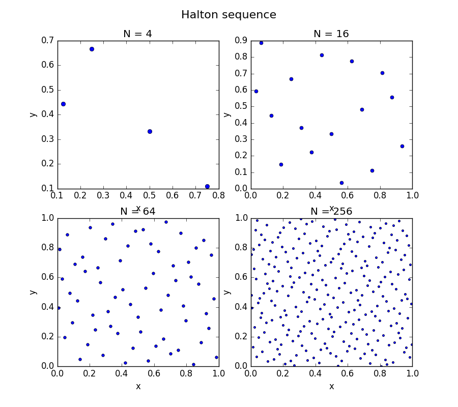
Figure: Example of a Halton sequence design

Configuration

Halton sequence technique generates points sequentially (see Sequential vs Batch). The user can ask GTDoE to leap over elements of the sequence and skip first several elements of the sequence, i.e. generate sample \(X = \{\vec{x}_s, \vec{x}_{s + (l + 1)}, \vec{x}_{s + 2 \cdot (l + 1)}, \ldots, \vec{x}_{s + n \cdot (l + 1)}\}\), where values \(s\) and \(l\) are skip and leap values defined by GTDoE/Sequential/Skip and GTDoE/Sequential/Leap options.

7.2.1.8. Sobol Sequence

Sobol sequence is another low-discrepancy sequence. Its construction is based on the theory of finite fields.

Let \(2^m\) be fixed upper bound for a number of points in a sequence. First of all, we need \(n\) different irreducible polynomials \(p_i \in F_2[x]\), where \(F_2[x]\) is the finite field with two elements. Let \(p_i(x)\)

\[p_i (x) = x^r + a_1x^{r-1} + \ldots + a_{r-1}x + 1\]

Let \(v_j, j \in [1, r]\) is arbitrary direction numbers such that \(1 \le \frac{v_j}{2^{m-j}}\le 2^j - 1\) and \(\frac{v_j}{2^{m-j}}\) is an odd integer. Then for \(j = r+1, \ldots, m\) we compute remaining direction numbers as

\[v_j = a_1v_{j-1} \oplus a_2v_{j-2} \oplus \ldots \oplus a_{r-1}v_{j-r+1} \oplus v_{j-r} \oplus \frac{v_{j-r}}{2^r},\]

where \(\oplus\) is the bit-by-bit exclusive-or operator.

Once we have computed all \(v_j, j \in [1, m]\) we can compute \(x^i_k, i \in [1, n]\) by a recurrent relation:

\[x^i_k = \frac{x^i_{k-1}2^m \oplus v_c}{2^m}, c = \min \{j\, | b_j = 1\},\]

where \(b_j\) are the coefficients in binary representation of \(k\).

Maximal dimensionality for current implementation of Sobol sequence is \(1111\).

• Pros
  • One of the most effective low-discrepancy sequences for Monte Carlo experiments
  • Can always be extended by more points
• Cons
  • High dimensional projections are still correlated (however, less than in Halton’s construction)

Configuration

Sobol sequence technique generates points sequentially (see Sequential vs Batch). The user can ask GTDoE to leap over elements of the sequence and skip first several elements of the sequence, i.e. generate sample \(X = \{\vec{x}_s, \vec{x}_{s + (l + 1)}, \vec{x}_{s + 2 \cdot (l + 1)}, \ldots, \vec{x}_{s + n \cdot (l + 1)}\}\), where values \(s\) and \(l\) are skip and leap values defined by GTDoE/Sequential/Skip and GTDoE/Sequential/Leap options.

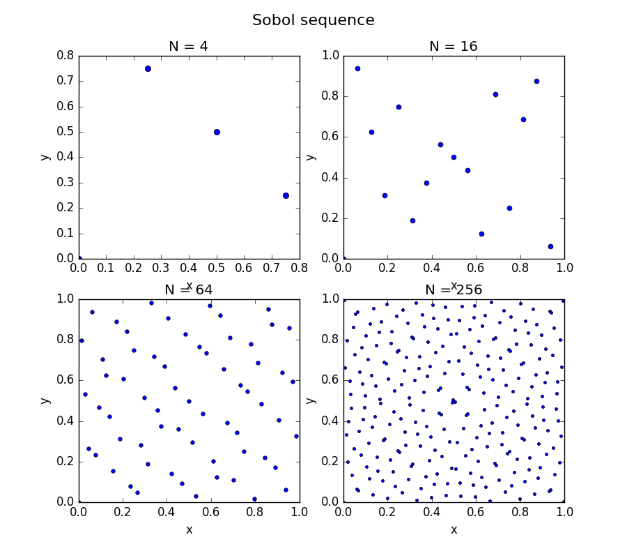
Figure: Example of a Sobol sequence design

7.2.1.9. Faure Sequence

Faure sequence is a low-discrepancy sequence with one of the best theoretical discrepancy bounds.

First let \(p\) be the smallest prime number such that \(p \geq d\). It would be convenient to set an a priori upper bound \(p^m\) for a number of points in a sequence and to precompute for all \(i,j\) with \(0 \leq i \leq j \leq m\) the binary coefficients modulo \(p\) : \(c_{ij} = {j \choose i} \mod p\).

Now for any \(n < p^m\) we define \(x_n\). Let \(n = \sum _{j = 0}^{\hat{m}-1}p^j b_j\) be the \(p\)-adic representation of \(n\), \(b_j \in \{0, \ldots, p - 1\}\) and \(\hat{m} = \max \{j \ | \ b_j > 0\}\). Then for the first variable we get: \(x_n^1 = \sum _{j=0}^{\hat{m}-1} b_j p^{-j-1}\) For all remaining variables (\(k = 2, \ldots, d\) in natural order):

\begin{align} \bar{b_j} &= \sum _{l=j}^{\hat{m}-1} c_{jl} b_l \bmod{p},\ j \in \{0, \ldots, \hat{m} - 1\}\\ b_j &= \bar{b_j},\ j \in \{0, \ldots, \hat{m} - 1\}\\ x_n^k &= \sum _{j=0}^{\hat{m}-1} \frac{\bar{b}_j}{p^{j+1}} \end{align}

• Pros
  • One of the best discrepancy upper bounds
  • Can always be extended by more points
• Cons
  • Most computationally expensive one of the implemented low-discrepancy sequences

Configuration

Faure sequence technique generates points sequentially (see Sequential vs Batch). The user can ask GTDoE to leap over elements of the sequence and skip first several elements of the sequence, i.e. generate sample \(X = \{\vec{x}_s, \vec{x}_{s + (l + 1)}, \vec{x}_{s + 2 \cdot (l + 1)}, \ldots, \vec{x}_{s + n \cdot (l + 1)}\}\), where values \(s\) and \(l\) are skip and leap values defined by GTDoE/Sequential/Skip and GTDoE/Sequential/Leap options.

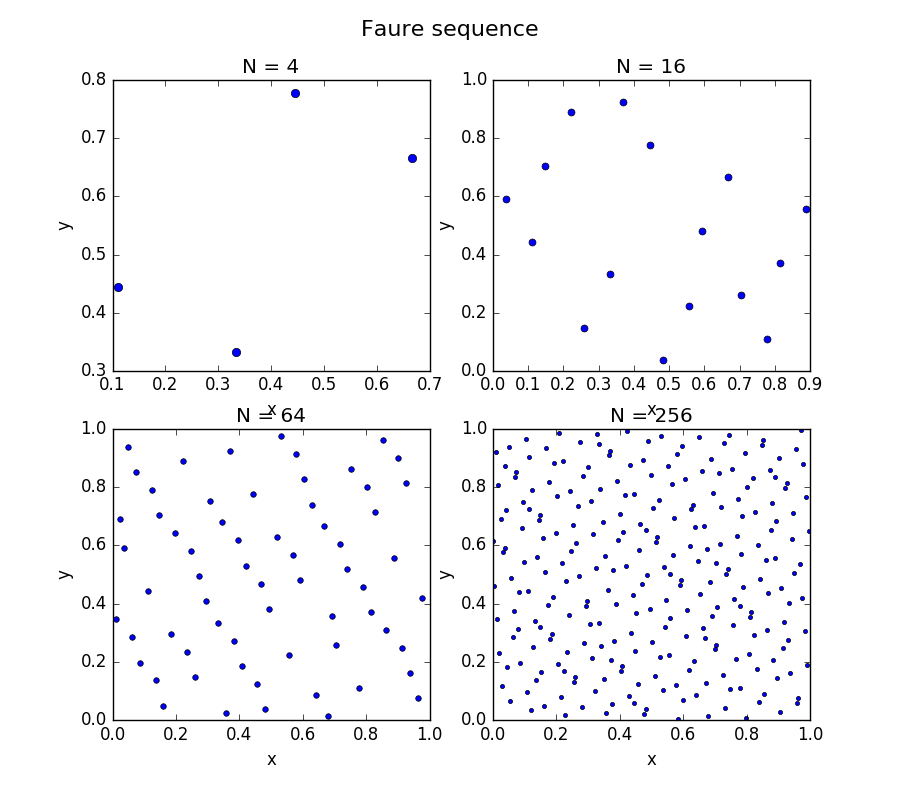
Figure: Example of a Faure sequence design

7.2.1.10. Orthogonal Array

Orthogonal Array (OA) in GTDoE is a fractional factorial type technique designed to work with categorical (discrete) variables. As every other fractional factorial technique, OA can be applied when the number of variables and their levels is too large for exhaustive (full factorial) testing. OA can also be understood as a generalization of Latin hypercube sampling (LHS). Similarly to LHS, orthogonal array generation involves permutations of variables’ levels. The array generation algorithm selects permutations which reduce possible correlation of responses and therefore increase the amount of information obtained when evaluating an orthogonal array DoE.

Orthogonal array generation requires variables with predefined levels. The OA technique can either assign levels to variables automatically or get levels defined by the GTDoE/OrthogonalArray/LevelsNumber or GTDoE/CategoricalVariables options.

• Use GTDoE/OrthogonalArray/LevelsNumber to specify the number of levels for each variable. OA will generate levels as specified, distributing them uniformly in each variable’s value range defined by the lower and upper bounds.
  • If you want to specify a non-uniform distribution of levels for some variable, add it to the GTDoE/CategoricalVariables option and set values of its levels explicitly. In this case, both options should be set accordingly — for example, if GTDoE/CategoricalVariables defines 5 levels for some variable, then GTDoE/OrthogonalArray/LevelsNumber should also set the number of levels for this variable to 5.
• You can specify GTDoE/CategoricalVariables and leave GTDoE/OrthogonalArray/LevelsNumber default (unset). In this case, the OA technique uses specified levels for variables included in the GTDoE/CategoricalVariables option, and assigns levels to all other variables automatically.
• If both options are default (unset), the OA technique automatically assigns levels to all variables to generate an OA which is as close as possible to the requested sample size.

The orthogonal array definition imposes specific sample size restrictions depending on the number of variables and the number of levels for each: there is a minimum sample size, and the number of points to generate can be increased only in certain increments, up to the maximum size which is equal to the size of a full factorial design. As a workaround for these limitations, the OA technique can generate different array types explained in the Array Types and Requirements section. Additional types are “nearly orthogonal” arrays which may violate some OA requirements to lower the minimum size limit and the increment size, or to generate a sample of arbitrary size.

Generating an orthogonal array which would conform to all restrictions and have good space-filling properties is a non-trivial combinatorial optimization problem. The OA technique solves it using an algorithm which can start from multiple initial guess — that is, perform multistart optimization. The maximum allowed number of additional starting points is controlled with the GTDoE/OrthogonalArray/MultistartIterations option. For large samples, OA generation is time-consuming due to the \(\mathcal{O}(n^3)\) complexity of the generation algorithm (\(n\) is the sample size). In such cases GTDoE/OrthogonalArray/MultistartIterations provides a certain trade-off between the generation time and DoE quality.

7.2.1.10.1. Definition

Consider a \(d\)-dimensional design space with variables \(x_i\), \(i = \{1, \dots, d\}\) where each variable takes values from a predefined set containing \(s_i\) elements (levels of the variable): \(x_i = \{x_{i,1}, \dots, x_{i,s_i}\}\), \(s_i\) is the number of levels. An orthogonal array sample satisfies the following requirements:

• Representativity: for each \(x_i\), all levels of \(x_i\) are found in the sample.
• Balance: for each \(x_i\), each of its levels \(x_{i,k}\) appears in the sample the same number of times.
• Two-strength: for each pair of variables \(x_i\), \(x_j\), \(i \neq j\) each unique combination of their levels \((x_{i,m}, x_{j,k})\), \(m = \{1, \dots, s_i\}, ~ k = \{1, \dots, s_j\}\) appears in the sample the same number of times.
• No dupes: there are no duplicated design points — that is, a unique combination of levels of the entire set of \(d\) variables \((x_{1,l_1}, \dots, x_{d,l_d})\), \(l_i = \{1, \dots, s_i\}\) is never found in the sample twice.

These requirements are compatible with the classic definition of a 2-strength simple orthogonal array (an orthogonal array is simple if it does not contain any repeated rows). The difference is that GTDoE allows for variables with different number of levels \(s_i\).

7.2.1.10.2. Array Types and Requirements

The OA definition imposes very specific restrictions on the array size — that is, the requested sample size set by the count argument to generate(). For an array which fully conforms to the above definition (a proper orthogonal array), these limits are:

• The minimum size of a proper OA is \(N_{min} = LCM(s_i \cdot s_j, i \neq j)\) — the least common multiple of all pairwise products of the level set sizes for different variables.
• The maximum size of a proper OA is \(N_{max} = \prod_{i=1}^d s_i\), which is the size of a full factorial design.
• The size of a proper OA can be increased only in \(N_{min}\) increments: \(N_{OA} = k N_{min}\), \(k = \{1, \dots, N_{max}/N_{min}\}\).

If the requested sample size \(N\) is less than \(N_{min}\), OA generation fails. If \(N\) is not a multiple of \(N_{min}\), the OA size is automatically adjusted to the closest increment which does not exceed \(N\): if \(k N_{min} \lt N \lt (k+1) N_{min}\), then \(N_{OA} = k N_{min}\).

Note

An orthogonal array is easier to generate when all variables \(x_i\) have the same number of levels \(s_i\), or when these numbers have a common divisor, preferably equal to one of \(s_i\). Also, when all \(s_i\) are coprime numbers, the only possible orthogonal arrays are full factorial and an irregular array.

To work around some of the above restrictions, the OA technique provides an option to generate a “nearly orthogonal” array (NOA) which is less restrictive in terms of the array size but deviates from the OA definition. There are the following NOA types which you can enable with the GTDoE/OrthogonalArray/ArrayType option:

• Balanced NOA: an array which may violate the two-strength requirement — that is, pairwise combinations of variables’ levels may appear in the array different number of times. For this type \(N_{min} = max(s_i)\) (the greatest number of levels). Similarly to a proper OA, the size of a balanced NOA is a multiple of \(N_{min}\), and the requested sample size is automatically adjusted to the closest possible increment.

  When this type is selected, the OA technique generates a proper orthogonal array when possible (for large enough \(N\)), and the two-strength requirement is violated only if \(N\) is not sufficient to generate a proper orthogonal array for the given number of variables and their levels. This behavior makes balanced NOA suitable for many cases, hence it is the default array type for the OA technique since pSeven Core 6.16.

• Irregular NOA: an array which is a fraction of a proper OA but may violate any of the OA requirements. This type has no lower limits for array size and increment size (\(N_{min} = 1\)), so the sample can have any size. Nevertheless the level permutations are selected using the same criteria as in proper OA generation, so an irregular NOA may provide a more representative DoE than random or LHS for the same sample size \(N\).

  With increasing \(N\), irregular NOA improves to a balanced NOA, and finally to a proper OA. That is, even if you set the type of array to irregular NOA, the OA technique prefers to generate a balanced NOA or a proper OA if \(N\) is large enough.

Note that (by definition) the maximum size for all array types is the size of a full factorial design: \(N_{max} = N_{FF} = \prod_{i=1}^d s_i\), where \(d\) is the number of variables and \(s_i\) is the number of levels for each. You can take advantage of this feature to generate a full factorial Doe with preset levels: specify levels for all variables using the GTDoE/OrthogonalArray/LevelsNumber or GTDoE/CategoricalVariables option, and specify an arbitrary high sample size to allow the OA technique to generate all possible combinations of levels.

7.2.2. Optimal Designs for Response Surface Models

Optimal Designs for Response Surface Models (RSM) are DoEs which are constructed by optimizing some criterion that results in minimizing either

• the generalized variance of the parameter estimates, or
• variance of prediction

for a pre-specified RSM model structure (linear, quadratic, etc., see RSM). As a result, the optimality of a given Optimal Design is model dependent.

That is, the user needs to specify a model structure (for example, to specify that the model is quadratic with categorical input variables) before the actual experiments. Given the total number of experimental runs and a specified model structure, the optimization procedure chooses the optimal set of design points from a candidate set of possible design points. This candidate set of design points usually consists of all possible combinations of various levels of input variables. In contrast to space-filling designs, optimal designs seek not only to place points in the design space uniformly, but also to achieve more robust and consistent estimates of RSM parameters or its predictions.

Optimal RSM designs are suitable for specific cases when two assumptions hold:

1. Sample size constraints are too restrictive for classical approaches.
2. Response Surface Model structure is known a priori, before any experiments.

Such designs allow to robustly estimate specific Response Surface Model using the limited number (usually very small) of actual experiments.

• Pros
  • Provides best possible estimators for the Response Surface Models
  • Requires smaller number of experimental runs than classical designs to achieve the same model accuracy
  • Guarantees no correlation among regressors for the specified Response Surface Model structure
  • Can generate relatively small sample size designs with good statistical properties in contrast to classical approaches
  • Supports discrete and categorical variables
• Cons
  • Proven effectiveness only for the Response Surface Model with a priori specified structure
  • Non optimal for any Response Surface Model with the structure other than the specified one

7.2.2.1. Criteria Optimization Based Designs

Such design is generated by optimizing one of the optimality criteria.

Let \(B\) be a design space and \(X = \{{x}^i\}_{i=1}^{N} \subset B\) be a DoE. Variances of parameters can be estimated via least squares as \(\mathrm{Var}(\hat{\mathbf{c}}|X)=\sigma^{2}(\psi(X)^{T}\psi(X))^{-1}\), where \(\sigma^{2}\) is a noise variance and \(\psi(X)\) is a full RSM design, i.e. \(\psi(X) = \{ \psi(x^1), \ldots, \psi(x^N)\}\).

Two types of optimality criteria are currently implemented in GTDoE:

1. D-optimal design minimizes determinant of design inverse covariance matrix, i.e. finds such design \(X\), that

   (1)\[\mathrm{det[}(\psi(X)^{T}\psi(X))^{-1}]\rightarrow \min_{X}.\]

   This approach allows minimizing variance of parameters estimates. “D” stands for Determinant optimality.

2. IV-optimal design minimizes the integrated variance of the prediction throughout the design space, i.e. finds such design \(X\), that

   (2)\[\int_{B}\psi(x)(\psi(X)^{T}\psi(X))^{-1}\psi(x)^{T}dx \rightarrow \min_{X}.\]

   “IV” stands for Integrated Variance optimality.

The generic optimization procedure for solving (1) and (2) is based on the Fedorov algorithm and consists of the following steps:

1. Define the number of levels for each variable based on the RSM type as the maximum power of this variable in the model plus 1. Note that this holds only for numerical variables as levels for categorical variables are determined beforehand.
2. Generate full-factorial design consisting of all combinations of numerical variables levels, obtained in the previous step, and categorical levels. This set is called a candidate set for design.
3. Take the required number of points from the candidate set at random and calculate optimality criterion for these points.
4. Proceed with optimization via including and excluding points from the design in order to minimize the value of criterion specified. New points are drawn from the candidate set.

Configuration

The user can specify the type of RSM model by setting GTDoE/OptimalDesign/Model. The type of optimality criteria is defined by GTDoE/OptimalDesign/Type. The option GTDoE/OptimalDesign/Tries allows performing multistart optimization, i.e. performing optimization several times using different random subsets in step 4 of the algorithm above and then choose the best generated subset in terms of optimality criteria.

7.2.2.2. Box-Behnken

Box-Behnken design is an alternative approach to generate designs for RSM construction. It has the following properties:

• Each variable takes at least three different equally spaced values.
• Number of points in design makes it possible to construct RSM with estimation of coefficients being accurate enough. This requirement imposes limitation on a ratio of the number of coefficients in quadratic model to the number of generated points.
• Variance estimation for RSM prediction depends roughly only on the distance to the center. For points which belong to the smallest hypercube containing the generated DoE we want the variance to be almost the same.

To achieve these goals and generate the full Box-Behnken design we use the following algorithm:

1. For each variable define three levels (low, mean, high). For continuous variable low and high level are defined by low and upper bound for this input variable correspondingly, mean level equals half-sum of lower and upper bound for this variable. For categorical input variable low and high levels are defined by min and max values of categorical variable, mean level equals median of all possible categorical variable values.

2. Then for all pairs of variables \((i, j)\) generate two-level design: fix all variables except \(i\)-th and \(j\)-th at mean values, for selected pair of variables generate four points with (low, low), (low, high), (high, low), (high, high) \(i\)-th and \(j\)-th variables values:

   \((mean, \ldots, mean, \underbrace{low}_i, mean, \ldots, mean, \underbrace{low}_j, mean, \ldots, mean)\),

   \((mean, \ldots, mean, \underbrace{low}_i, mean, \ldots, mean, \underbrace{high}_j, mean, \ldots, mean)\),

   \((mean, \ldots, mean, \underbrace{high}_i, mean, \ldots, mean, \underbrace{low}_j, mean, \ldots, mean)\),

   \((mean, \ldots, mean, \underbrace{high}_i, mean, \ldots, mean, \underbrace{high}_j, mean, \ldots, mean)\).

3. Add point with all mean variables values: \((mean, \ldots, mean, mean, mean, \ldots, mean, mean, mean, \ldots, mean)\).

Configuration

The full Box-Behnken design is comprised of \(2 d (d - 1) + 1\) (\(d\) is specified input dimension) points. If specified number of generated points is not big enough to generate the full Box-Behnken design we select large enough number of input variables pairs and do not generate \(4\) corresponding points for each of these randomly selected pairs of input variables. Moreover, if the number of points to generate minus \(1\) can not be divided by \(4\), for one randomly selected pair we generate not all \(4\) points, but small enough number of points to obtain the desired sample size. To force GTDoE to generate full Box-Behnken DoE regardless of specified DoE size the user can set GTDOE/BoxBehnken/IsFull to True.

Note, that Box-Behnken technique has the following limitations:

• We can not generate design for input dimension \(d\) smaller than \(3\).
• Each categorical variable has to include at least \(3\) different levels (so, we can define mean level for this input variable).

7.2.3. Adaptive Design of Experiments

7.2.3.1. Overview

It is common in surrogate modeling when design of experiments is not given a priori and one may want to select design in some optimal way. The first option to do this is to use one of Space-Filling DoE techniques. The other option is to generate initial design by one of space-filling techniques, construct approximation based on this sample and then enrich sample iteratively adding points. Two main motivations for such a workflow are the following:

• Approximation of a target function contains information about its behavior. Thus, one can expect that this information can help to choose additional sample locations in a way which benefits most to quality of approximation.
• Adaptive enrichment of the training set allows to flexibly control the number of points in it. If the desired quality of approximation is achieved the process can be stopped. It is especially important when the target function is heavy, which means that every function evaluation is very time-consuming.

An important issue arises, if initial design is given, but it can not provide accurate enough approximation. In this case, it is necessary to generate additional design which supplements the existing one, so the quality of a surrogate model built based on a union of an old design and a new one is as high as possible.

Another problem that can be solved by Adaptive DoE is to complement existing design to make it more uniform.

An adaptive DoE technique is a method which iteratively adds points to the training set and constructs corresponding approximations given maximum number of target function evaluation (budget). In current version of GTDoE one can perform adaptive design of experiments with and without blackbox for the target function provided. In the second case one requires an initial sample of points and corresponding function values.

7.2.3.2. Problem Statement

Let \(f(\cdot): \mathbb{R}^d \rightarrow \mathbb{R}\) a given function that we want to approximate inside a given box \(B \subset \mathbb{R}^d\). The goal is to generate DoE \(X\), such a surrogate model \(\hat{f}(\cdot)\) constructed using the set of designs \(D = \{(x^i, f(x^i))\}_{i = 1}^{N}\) is as accurate as possible. The tool distinguishes two cases: when blackbox for the target function is provided, and we can evaluate it in new generated points, and when only an initial sample is provided.

We start with the problem statement for the case with provided blackbox for the target function. We suppose that blackbox allows calculating \(f(x)\) in any point \(x\) from the box \(B\). The initial training set \(D_{in} = X_{in} \times Y_{in} = \{(x^i, f(x^i))\}_{i = 1}^{N_{in}}\) can be specified by the user or generated by one of Space-Filling DoE techniques. Then for a given budget of target function evaluations \(K\) additional training points are generated by batches of \(k\) points until the budget is exhausted. The final training set is \(D_N = X_N \times Y_N = \{(f(x^i), x^i\}_{i = 1}^{N}\).

The input and output for the adaptive DoE are

• Input

  • budget \(K\);
  • blackbox for \(f(\cdot)\);
  • initial training set \(D_{in}\) (optional, either contains only inputs \(X_{in}\) or both inputs and outputs \((X_{in}, Y_{in})\));
  • options.

• Output

  • final designs \(D_N\).

The problem statement described above is rather general, but it is often the case that one can not provide the target function \(f(\cdot)\) blackbox to a design generation algorithm. For example, one obtains a new value of the target function using an experiment in a wind tunnel or some kind of a field experiment. Adaptive design of experiments allows gaining benefits from previously obtained sample \(D_{in}\) even if a blackbox for \(f(\cdot)\) is not provided. Input and outputs for adaptive DoE in this case are:

• Input

  • number of points to generate \(K\);
  • initial training set \(D_{in}= (X_{in}, Y_{in})\) (or \(X_{in}\) but in this case only Uniform criterion is available);
  • options.

• Output

  • final DoE \(X_N\).

Note, that after run of adaptive DoE of this kind one obtains \(X_N\) and is able to calculate \(Y_N\), he/she can pass updated sample \(D_N = (X_N, Y_N)\) to adaptive DoE algorithm and obtain new points. This process looks like one described at the beginning of this subsection, but in this case it requires additional unavoidable manual work, because the algorithm has no direct access to the target function \(f(\cdot)\).

As the first case with the provided target function \(f(\cdot)\) is the most common we consider it in details below.

7.2.3.3. Toy Example

Suppose the function to be approximated is:

\[f(x) = (6 x - 2)^2 \sin(12 x - 4).\]

Suppose we know function values only at points \(X = \{0.0111, 0.2718, 0.4383, 0.7511, 0.9652\}\). We train approximation of the function using values at points \(X\). The approximator based on Gaussian processes gives us not only the approximation \(\hat{f}(\cdot)\), but also expected error of approximation \(\hat{\sigma}(\cdot)\) (see details). In this case we can use the following workflow:

• evaluate function \(f(\cdot)\) in the point of maximum expected error;
• add this point and the corresponding function value to the training set;
• construct new approximation.

By doing so one can expect that adding points in the region with high uncertainty of prediction will lead to better approximation.

Results of five iterations of such an algorithm are given in the figure below. One can see that every iteration of the algorithm significantly increases the quality of approximation. Finally, we obtain very accurate resulting approximation.

Figure: Example for model function. Blue line is the function \(f(\cdot)\), red line is the approximation \(\hat{f}(\cdot)\), green line is \(\hat{\sigma}(\cdot)\) (Accuracy Evaluation) predicted on current iteration. Training sample points are shown as blue squares, new point selected by adaptive DoE algorithm is the red circle.

• Note: This image was obtained using an older pSeven Core version. Actual results in the current version may differ.*

7.2.3.4. Adaptive DoE Workflow

The workflow with the adaptive DoE includes the following elements.

• Generation of initial training set (if initial training set was not set by user).

• Main adaptive DoE cycle. The following steps are performed iteratively while the budget of target function evaluations is not exhausted:

  • Construction of approximation model. At this step, approximation is constructed on base of the current training set. Internal validation can also be performed at this stage.
  • Generation of adaptive DoE points. At this step, new train points are computed as ones maximizing some adaptive DoE criterion.

7.2.3.4.1. Generation of the initial training set

There are several possibilities of specifying the initial training set for adaptive DoE:

1. Initial training set \(D_{in} = (X_{in}, Y_{in}) = \{(x^i, f(x^i))\}_{i = 1}^{N_{in}}\) can be specified by the user.
2. The user can specify only \(X_{in} = \{x^i\}_{i = 1}^{N_{in}}\). In this case, \(Y_{in} = \{f(x^i)\}_{i = 1}^{N_{in}}\) is computed by solver \(f(x)\) and corresponding number of function evaluations \(N_{in}\) is subtracted from the budget.
3. The user can just specify \(N_{in}\) (in default \(N_{in} = 2d + 3\)) and Space-Filling DoE techniques method (by default Latin Hypercube Sampling). In this case, \(X_{in} = \{x^i\}_{i = 1}^{N_{in}}\) is generated by chosen space-filling DoE technique and \(Y_{in} = \{f(x^i)\}_{i = 1}^{N_{in}}\) is computed by the solver \(f(\cdots)\). Corresponding number of function evaluations \(N_{in}\) is subtracted from the budget.

7.2.3.4.2. Construction of approximation model

Building the approximation model is a crucial part of adaptive DoE process. Good quality of approximation ensures that adaptive DoE techniques work well. Also, it is very desirable that approximator can model expected errors of approximation, because many adaptive DoE techniques require such an estimation. Both these properties meet in approximators based on Gaussian processes (GP) technique.

GTDoE can estimate the accuracy of constructed model using Internal Validation (IV) procedure. The result of this procedure is written to the log file and to the constructed model’s info file. The procedure can be turned on/off by the GTDoE/Adaptive/InternalValidation option (the default value is off).

7.2.3.4.3. Generation of adaptive DoE points

Once approximation \(\hat{f}(\cdot)\) based on training set \(D_N\) is constructed, adaptive DoE points can be generated. These points are generated as ones maximizing some adaptive DoE criterion \(g(x | \hat{f}, D_N)\). Optimizing of the criterion is performed by means of global optimization algorithm Simulated Annealing. Thus, this optimization algorithm solves following optimization problem:

\[x_{new} = \arg\min_{x \in \mathbb{X}} g(x | \hat{f}, D_N).\]

Then solver value \(f_{new} = f(x_{new})\) is evaluated and the number of function evaluations left (budget) is reduced by one. Pair \((x_{new}, f_{new})\) is added to the training set \(D_{N + 1} = D_N \bigcup (x_{new}, f_{new})\). The process continues iteratively until the budget is exhausted.

7.2.3.5. Criteria

There are three main adaptive DoE criteria which are implemented in GTDoE, namely:

• Uniform. This criterion samples points which are far from existing training points. It actually doesn’t depend on function values and on approximation.
• Maximum Variance. This criterion samples points with high uncertainty of prediction, i.e. points where the expected error of prediction is maximal (see Accuracy Evaluation for details).
• Integrated Mean Squared Error Gain - Maximum Variance. This criterion combines expected integrated error over all the experimental domain with Maximum Variance criterion. Next step look ahead error prediction and usage of integrated error allows selecting point which benefits most to quality of approximation. But this criterion is the most computationally demanding.

7.2.3.5.1. Uniform

This criterion selects points which are far from existing training points in terms of Euclidean distance. The criterion looks like:

\[\mathrm{uniform}(x) = \min\limits_{u \in X_N} d(x, u),\]

where \(d(x, u) = \sqrt{\sum_{i = 1}^n (x^{(i)} - u^{(i)})^2}\) is the Euclidean distance between points \(x\) and \(u\).

7.2.3.5.2. Maximum Variance

This criterion samples points with high uncertainty of prediction, i.e. points where the expected error of prediction is maximal (see Accuracy Evaluation for details).

\[\mathrm{maxVar}(x) = \hat{\sigma}^2(x | X_N).\]

7.2.3.5.3. Integrated Mean Squared Error Gain – Maximum Variance

This criterion combines expected integrated error over all the experimental domain with Maximum Variance criterion. Next step look ahead error prediction and usage of integrated error allows criterion to select point which benefit most to quality of approximation, but also it is more computationally demanding than other criteria:

\[ \begin{align}\begin{aligned}\mathrm{integratedMseGainMaxVar}(x) =\\=\frac{\hat{\sigma}^2(x | X_N)}{|\mathbf{X}|} \int_{\mathbf{X}} \bigr(\hat{\sigma}^2(u | X_N) - \hat{\sigma}^2(u | X_N \cup x)\bigl) d u,\end{aligned}\end{align} \]

where \(\hat{\sigma}^2(u | X_N \cup x)\) is expected error at point \(u\), if point \(x\) is added to the training set.

7.2.3.6. Configuration

1. Generation of initial training set.

   In sample based mode the user can provide its own initial sample by initializing Generator with additional parameters init_x and init_y – input points and responses at these points.

   If the user doesn’t have the initial sample, GTDoE will generate it itself. The size of initial DoE in this case and the type of DoE are specified by the options GTDoE/Adaptive/InitialCount and GTDoE/Adaptive/InitialDoeTechnique.

2. Construction of approximation model.

   Adaptive GTDoE techniques (all except Uniform criterion) use a surrogate model to generate DoE. Building a surrogate model can be a time-consuming process. The user can control construction time by setting GTDoE/Adaptive/Accelerator. This option is identical to GTApprox option GTApprox/Accelerator.

   The user can ask GTDoE to build a surrogate model which fits the initial and generated data exactly, i.e. the predictions of the surrogate model at the initial and generated points equal the true responses at these points. This is achieved by setting GTDoE/Adaptive/ExactFitRequired to True. Exact fit can be useful if it is known that responses do not contain noise. Otherwise, the quality of a surrogate model and, therefore, generated DoE can be poor.

   The quality of constructed surrogate models can be controlled. For this purpose, enable GTDoE/Adaptive/InternalValidation option. Note that Internal Validation is rather time-consuming procedure and enabling it can significantly increase the time of DoE generation.

3. Generation of adaptive DoE points.

   The type of criterion to be used for generation of adaptive DoE is specified by GTDoE/Adaptive/Criterion.

   There are several options controlling optimization of the criterion.

   GTDoE/Adaptive/AnnealingCount – sets the number of evaluations of the criterion during optimization. Increasing this number improves the results of DoE but can also increase the time elapsed for generation.

   By default Adaptive DoE generates points iteratively. At each iteration the tool builds a surrogate model using the initial sample and already generated sample. And then using this model chooses a new point. Such a procedure is time-consuming. The user can set the number of points to generate at each iteration by setting GTDoE/Adaptive/OneStepCount. One can also specify GTDoE/Adaptive/TrainIterations – the number of adaptive DoE iterations between rebuilds of approximation model. This speeds up the generation procedure at the cost of worse DoE.