3.3. Supported Problem Types

This page provides a brief summary of methods implemented in GTOpt.

3.3.1. Overview

1. General purpose methods, used in most algorithms below.

• Determination of steepest, Quasi-Newton, and quadratically-constrained direction, and the magnitude of optimal descent.
• Pool of one-dimensional line search methods.
• Specialized linear equations solver aimed at saddle-point systems.
• Universal problem transformations respecting complete independence of all representations and hence the parallelism of execution.

2. Noisy data handling techniques.

   Needed to fight with usually present in engineering applications noise in problem observables. Implemented at lowest level therefore none of upper level algorithms (notably gradient-based) should care about problem noisiness.

3. Mathematical programming: mixed-integer linear programming (MILP).

   External solvers are used. Current default is CBC/CLP.

4. Mathematical programming: quadratic programming (QP).

Original implementation, works for both definite and indefinite problems, suitable for engineering applications and is a prime solver for internally generated subproblems.

5. Mathematical programming: unconstrained non-linear programming (UNLP).

• Nonlinear simplex, nonlinear conjugate gradients, all with original implementation and appropriate adaptations for engineering settings.
• Derivative-free Powell method, again original implementation with a proper account for engineering specifics.
• Quasi-Newton family of methods with various update and search strategies.

6. Mathematical programming: constrained non-linear programming (NLP).

• Sequential quadratic programming with filtering (no merit functions).
• Sequential quadratically constrained quadratic programming with filtering, as far as we know has no analogs.

All methods are adopted to handle engineering specific issues (noise, implicit constraints, and other).

7. Constraint satisfaction problems (CSP).

   Works via reformulation of CSP in term of auxiliary NLP, hence uses the above pool of NLP methods.

8. Multi-objective optimization: single solution finding.

   In many cases the whole Pareto frontier is not really needed, it is enough to get the nearest to current guess Pareto optimal solution. Methods of this family realize required functionality using in-house developed methods of multi-objective steepest and Quasi-Newton descent direction finding.

9. Multi-objective optimization.

   Original gradient-based implementation, avoids altogether evaluations far away from Pareto variety and in this sense is a “local” search algorithm. As far as we know this is the only implementation of local multi-objective optimization.

10. Surrogate based optimization (SBO): constrained single-objective problems.

    Based upon widely known probability improvement approach using Gaussian processes (GP) methodology to construct surrogate models. However, the algorithm is sharply different from available implementations and avoids almost all deficiencies of probability improvement methods. Currently, utilizes custom GP modeling adopted for high problems dimensionality and other real-world applications issues. Additionally utilized in-house developed DoE strategy which respects as much as possible feasibility domain of the problem.

11. Surrogate-based optimization (SBO): constrained multi-objective problems.

    Built on top of single-objective SBO, utilizes Chebyshev convolution to sequentially discover Pareto frontier.

12. Global search methods, excluding SBO.

• Multi-start with SBO preconditioning: avoids too many initial points to be locally optimized via preliminary stage of SBO optimization. Highly efficient in local searches with multiple initial guesses.
• Random linkage: method is from the multi-start family of methods, however, uses various criteria to monitor problem multi-modality and to avoid unnecessary searches in simple problems. Due to relative expensiveness is utilized for internally generated subproblems only.

13. Robust optimization.

    Original implementation of robust optimization supporting both expectation-like and probability-type observables. Highly efficient due to the utilized adaptive sample selection strategy. Supports both direct and SBO-inspired approaches so that it is suitable for expensive to evaluate problems.

To summarize: GTOpt efficiently supports virtually all optimization problems, including their respective robust counterparts.

3.3.2. Linear Problems

Generic formulation of supported linear optimization problems reads

\[\begin{split}\begin{array}{cl} \min\limits_x \, F \vec{x} & \mbox{K linear objectives} \\ \vec{c}_L \,\le\, A \, \vec{x}\,\le\, \vec{c}_U & \mbox{M linear constraints} \\ \vec{x}_L \,\le\, \vec{x}\,\le\, \vec{x}_U & \mbox{box bounds} \end{array}\end{split}\]

where it is assumed that design vector \(\vec{x}\) might contain an arbitrary mixture of continuous and integer design variables. The case of linear optimization and, in particular, the case of mixed integer programming, is quite special since. On the other hand, it seems that occasion of purely linear problems is sufficiently rare case in real-life applications. Taking that into account, GTOpt uses an improved implementation of a mixed-integer solver based on the COIN-OR CBC open source MILP solver.

3.3.3. Quadratic Problems

Generic formulation of supported quadratic optimization problems reads

\[\begin{split}\begin{array}{cl} \min\limits_x \, \frac{1}{2} \vec{x}^T \, H \, \vec{x} + \vec{g}^T \, \vec{x} & \mbox{single quadratic objective function} \\ \vec{c}_L \,\le\, A \, \vec{x}\,\le\, \vec{c}_U & \mbox{M linear constraints} \\ \vec{x}_L \,\le\, \vec{x}\,\le\, \vec{x}_U & \mbox{box bounds} \end{array}\end{split}\]

where design variables are assumed to be real-valued and no special assumptions are made about the Hessian matrix \(H\). Implemented algorithm belongs to the class of active-set methods in which all iterates remain feasible all the way down to the solution (if it exists). It is partially based on Methods for Convex and General Quadratic Programming, P.Gill, E.Wong, 2010 and references cited in this paper. Technically, it utilizes functionality of numerical method mentioned in section Numerical Methods.

3.3.4. Box Constrained Single-Objective Problems

This is a special case of single-objective formulation in which no generic constraints are present.

\[\begin{split}\begin{array}{cl} \min\limits_x \, f(x) & \mbox{single generic objective function} \\ x^k_L \,\le\, x^k\,\le\, x^k_U & N\,\,\,\mbox{box bounds} \end{array}\end{split}\]

Numerous methods to solve this problem are widely known, however, virtually all of them do not fit our requirements. Namely, we should ensure algorithm stability with respect to usual in real-life applications issues: data noisiness, occurrence of undefined designs, maximal efficiency with respect to the number of underlying model evaluations etc. Therefore, all the methods listed below had been in-house implemented with serious modifications compared to other wide-spread realizations.

1. Powell method.

   Highly modified derivative-free method due to M.J.D.Powell (does not use derivatives explicitly).

2. Nonlinear conjugate gradients.

   Extremely robust method with cutting-edge update rules and line search procedures.

3. Quasi-Newton family.

   • Most powerful for smooth problems.
   • Automatic selection of normal or low-memory modes.
   • Efficient treatment of box bounds.

3.3.5. Single-Objective Constrained Problems

Single-objective constrained optimization is suitable for both analytic models and problems formulated on top of complex numerical simulation process. Moreover, depending on problem type and properties GTOpt automatically corrects the selection of best suited algorithms, which range from dedicated sequential quadratically constrained quadratic programming (SQCQP) for smooth underlying problems to more simple but robust derivative-free methods for noisy engineering applications.

Generic formulation of problems in question includes single objective functions subject to a number of most general constraints:

\[\begin{split}\begin{array}{cl} \min\limits_x \, f(x) & \mbox{single generic objective functions} \\ c^j_L \,\le\, c^j(x)\,\le\, c^j_U & M \,\,\, \mbox{generic constraints} \\ x^k_L \,\le\, x^k\,\le\, x^k_U & N\,\,\,\mbox{box bounds} \end{array}\end{split}\]

As it was in case of unconstrained optimization, numerous methods to solve this type of problems are widely known, however, none of them seems to fit our requirements. Therefore, GTOpt has a variety of suitable in-house developed methods, list of which is summarized below.

1. Method of multipliers.

   This is a highly customized implementation of widely known algorithm. Its prime application area within GTOpt in the solution of internally generated optimization subtasks because of inherent to it relatively large computations expensiveness (in term of number of functions evaluations).

2. Filter sequential quadratic programming (SQP)

   Powerful and most robust NLP algorithm available in GTOpt. Based on filtering philosophy (avoids merit functions altogether: does not ever mix objective and constraints). Internally utilizes functionality of optimal descent, outlined in section Numerical Methods.

3. Filter sequential quadratically constrained QP (SQCQP).

   Perhaps the only production implementation of SQCQP algorithms. Most powerful method for smooth problems. Utilizes filtering philosophy (like SQP). Heavily uses functionality of optimal and Quasi-Newton descent, outlined in section Numerical Methods.

3.3.6. Constraint Satisfaction Problems

These problems are the special instances of generic non-linear programming tasks, which objective functions are absent altogether (\(K=0\)). Therefore, the goal is to find any single feasible solution thus ensuring problem feasibility. In order to make the problem well-defined one usually considers artificial analytic objective, which slightly penalizes the distance (\(L_2\) or \(L_\infty\) depending on context) of current iterate from initial point \(x_0\).

\[\begin{split}\begin{array}{cl} \min\limits_x \, |x - x_0| & \\ c^j_L \,\le\, c^j(x)\,\le\, c^j_U & M \,\,\, \mbox{generic constraints} \\ x^k_L \,\le\, x^k\,\le\, x^k_U & N\,\,\,\mbox{box bounds} \end{array}\end{split}\]

The problem is solved via its reformulation as:

• either a constrained single-objective optimization problem (relaxation of imposed constraints)

  \[\begin{split}\begin{array}{c} \min\limits_{x,n,p} \, \epsilon |x - x_0| + \sum (n_i + p_i) \\ c^j_L - n^j \,\le\, c^j(x)\,\le\, c^j_U + p^j \\ x^k_L \,\le\, x^k\,\le\, x^k_U \\ n^k \ge 0 \,\,\, p^k \ge 0 \end{array}\end{split}\]

• or an unconstrained task of the type

  \[\begin{split}\begin{array}{c} \min\limits_x \, |\vec{\psi}|^2 \\ x^k_L \,\le\, x^k\,\le\, x^k_U \\ \end{array}\end{split}\]

(definition of constraints violation magnitude vector \(\vec{\psi}\) can be found in section Optimal Solution).

In either case the problem is solved by methods available in GTOpt (see Single-Objective Constrained Problems and Box Constrained Single-Objective Problems for details).

3.3.7. Multi-Objective Optimization

3.3.7.1. Overview

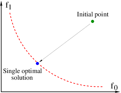
From very beginning it should be noted that multi-objective optimization (MO) could be understood in at least two different ways:

• Global MO: the aim is to find a whole variety of non-dominated points (Pareto frontier in objective functions space and respective Pareto set in design space).
• Local MO: purpose is to find a single non-dominated solution (perhaps, nearest to the initial guess).

The pictures below illustrate the key difference between these two approaches.

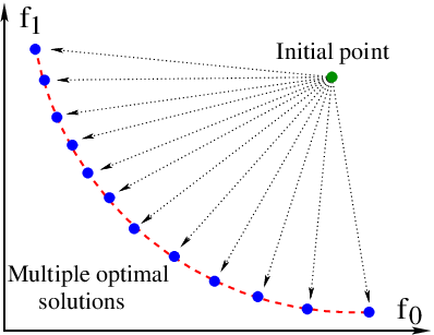
Methods implemented in GTOpt combine together local and global interpretations of MO to produce efficient algorithms of Pareto frontier discovery.

To motivate the approach used in GTOpt let us mention one of the main problems in solving multi-objective cases. Generically, Pareto set is not localized and methods, which are able to approximate whole Pareto frontier, have to be global. Usually this immediately implies the necessity to do evaluations far away from Pareto variety, which by-turn consumes too much computational resources.

The prime observation underlying GTOpt multi-objective optimization is that in the majority of cases Pareto optimal set could be described as union of compact (in objective space) continuous components each of which in case of continuous objective functions allows differential-geometric description. Therefore for single connected component it suffices to find any optimal point belonging to it and then perform incremental local spreading from known optimal solutions in the tangent plane to Pareto set. New points generated this way are not precisely optimal because Pareto set is not a hyperplane in general, however, the corresponding distance to optimality is small and hence required re-optimization efforts are minimal. As far as multiple connected components are concerned, their sequential discovery is in fact already built into the described strategy provided that single point optimization always finds nearest Pareto optimal solution: due to the negativity of Pareto front slopes in space of objectives the algorithm eventually discovers all connected components if it had been started from points minimizing each particular objective (anchor points).

Therefore, there are two prime ingredients of GTOpt multi-objective optimization:

• Local algorithm to reach Pareto optimal set. “Local” means finding nearest optimal solution.
• Pareto frontier discovery: spreading along optimal manifold (with re-optimization in case of curved Pareto set) with simultaneous maintenance of optimal points distribution evenness.

MO algorithms of GTOpt first look for small number of strictly Pareto optimal solutions. In theory, any optimal set could be used, but for reasons explained above (ability to discover all connected components) the most convenient points to start optimization with are the anchor points. By definition, for problem with K objectives there are exactly K anchors, \(k\)-th anchor is defined as minimizer of \(k\)-th objective function with no regard to other objectives (all relevant constraints remain imposed). As a by-product the set of anchor points also provides crude estimate of Pareto front extent along objective axes. Supplemented with user-provided number of optimal points to be finally generated this gives the minimal objective space distance to be used at spreading stage (see below).

Secondly, algorithm performs sequential spreading along the optimal manifold from all currently discovered optimal solutions. To this end Pareto set local geometry is reconstructed, prime purpose being to determine tangent plane at current optimal solution. Then algorithm generates a number of new (not optimal in general) points by shifting along basis axes of tangent plane from initial optimal position until the corresponding objective space separation becomes of required order (see above). If in the vicinity of proposed new position there are already discovered optimal solutions trial is discarded. Otherwise, new point is accepted and (if necessary) is pushed back to optimality. Process iterates until no unseen optimal solutions remain.

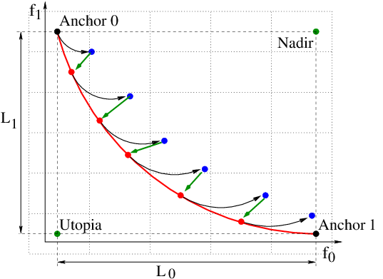
The whole process is qualitatively illustrated on the above picture; a few technical details of each stage are summarized below.

3.3.7.2. Technical Details

1. Anchor search stage.

   Proper determination of anchor points constitutes an essential part of the whole approach, however, technically it is almost equivalent to usual single-objective optimization and hence could be performed with standard algorithms of GTOpt (see Single-Objective Constrained Problems and Box Constrained Single-Objective Problems for details). Found anchors serve for estimation of Pareto frontier global geometry and as starting points for scattering process.

2. Re-optimization of scattered candidates.

   This is performed using either steepest or QN descent algorithms presented in section Numerical Methods. Due to the sufficiently small deviation from optimal variety pushing candidate solutions back to optimality is inexpensive procedure to which steepest and QN descent fit nicely.

3. Scattering process.

   To explain what is meant by local Pareto set geometry and how it is reconstructed, let us consider how optimal descent is found in unconstrained case \(M=0\). Constraint \(|d|_\infty \le 1\) could be traded for the term \(1/2 |d|^2\) in objective function. Then dualized optimal descent problem reads:

   \[\begin{split}\begin{array}{rlc} \min\limits_\lambda & \frac{1}{2}\,|\,\lambda_i \,\, \nabla f^i\,|^2 & \\ \mbox{s.t.~} & \sum\limits_i \, \lambda_i ~=~ 1\,, & \lambda_i \ge 0 \\ \end{array} \qquad d = - \sum\limits_i \, \lambda^*_i \,\, \nabla f^i\end{split}\]

with positive semi-definite Hessian \(G_{ij} = (\nabla f^i \cdot \nabla f^j)\). For locally optimal solution

\[G \lambda^* = 0\,, \quad \Longrightarrow \quad \mbox{rank}\,G \le K-1\]

and in general case we have \(\mbox{rank}\,G = K-1\), confirming that front dimensionality is \(K-1\). Therefore, one of eigenvectors of \(G\) determines optimal descent direction, which vanishes at locally optimal position (corresponding eigenvalue becomes zero as well). What are the remaining eigenvectors \(\lambda^{(\gamma)}\) of \(G\)?

In fact, one can show that

\[ t^{(\gamma)} ~=~ \mu^{-1/2}_{(\gamma)} \, \sum_i \, \lambda^{(\gamma)}_i \, \nabla f^i \qquad \gamma ~=~ 1, ..., K-1\]

provides an orthonormal basis in Pareto set tangent plane (Pareto front tangents are \(\lambda^{(\gamma)}\)). Here, \(\mu_{(\gamma)}\) are the corresponding eigenvalues, \(G \lambda^{(\gamma)} = \mu_{(\gamma)} \lambda^{(\gamma)}\).

The above construction generalizes trivially to the case of active constraints. Namely, let \({\cal P}_{\cal A}\) be an orthogonal projector onto the tangent plane to all active constraints (including active box bounds):

\[{\cal P}^2_{\cal A} = {\cal P}_{\cal A} \qquad {\cal P}_{\cal A} \, \nabla c^i = 0 \quad i \in {\cal A}\]

Then analysis of Pareto frontier local geometry goes through with the only change

\[\nabla f^i ~~ \to ~~ {\cal P}_{\cal A} \, \nabla f^i\]

To proceed we note that for infinitesimal shift in Pareto set tangent plane \(x = x^* + \epsilon \, t^{(\gamma)}\) sub-optimality of \(x\) is of order \(O(\epsilon)\). It then remains to push \(x\) back to optimal position which is rather cheap (we are still in the small vicinity of optimal set!). It remains to decide how to choose \(\epsilon\) in order to make the above approach practically sound.

Step size selection is by no means unique, the strategy adopted in GTOpt reduces to:

• End-user is required to provide single number \(N_f\) specifying how many points should appear on Pareto frontier.
• Method estimates the extent of Pareto frontier \(L_i\) along each axis in objective space (anchor search stage).
• Objective space is subdivided into non-overlapping boxes of size \(bb^i ~=~ L_i / N_f \qquad i = 1,..., K\).
• Ultimate goal is to finally have no more than one solution in each box.

Therefore, appropriate policy to select value of \(\epsilon\) parameter is as follows: objective space points \(f(x^*)\) and \(f(x^* + \epsilon \, t^{(\gamma)})\) should belong to the neighboring boxes.

3.3.8. Data Fitting Problem

Fitting involves finding coefficients (parameters) for one or more given models to known (e.g., experimental) data. In general, we want to minimize the distance between given data \(\left\{x^{model}_i, y^{model}_i\right\}_{i=1}^N\), produced, for instance, as results of measurement of a physical process, and theoretical results \(\left\{x^{model}_i, f(x^{model}_i, x)\right\}_{i=1}^N\) where \(f\) is a fitted model, \(x\) is vector of parameters of the model.

GTOpt has a special problem type ProblemFitting that helps formulate a fitting problem and reduces it to an optimization problem that allows invoking core optimization algorithm to fit the model.

To solve the fitting problem GTOpt reformulates it as minimization of residual. Mathematically, in the simplest case, this problem can be formulated as:

\[\min\limits_x \, \left(\frac{1}{N}\sum_{i=1}^N \left(f \left(x^{model}_i, x \right) - y^{model}_i \right)^2 \right)^{1/2}\]

GTOpt supports more general cases with weights on data, multiple multidimensional models and constraints on parameters:

\[\begin{split}\begin{array}{c} \min\limits_x \,\Biggl(\frac{1}{N M_1} \sum_{i=1}^{N} \sum_{k=1}^{M_1} \biggl[ w^{model_1}_{i,k} \left(f^{model_1}_{k} \left(x^{model_1}_{i}, x \right)-y^{model_1}_{i,k} \right) \biggr]^2 \Biggr)^{1/2} \\ \cdots \\ \min\limits_x \,\Biggl(\frac{1}{N M_m} \sum_{i=1}^{N} \sum_{k=1}^{M_m} \biggl[ w^{model_m}_{i,k} \left(f^{model_m}_{k} \left(x^{model_m}_{i}, x \right)-y^{model_m}_{i,k} \right) \biggr]^2 \Biggr)^{1/2} \\ L \le{x}\le{B} \\ L_c \le{c(x)}\le{B_c} \end{array}\end{split}\]

where \(\{model_l\}_{l=1}^m\) is a set of models each of which has out dimension \(M_l\), \(\left(w^{model_l}_{i_k}\right)\) is matrix of weights (for each model, for each point in input data), \(L\) and \(B\) are bounds on vector of parameters \(x\) and \(c(\cdot)\) is vector constraint on parameters with bounds \(L_c\) and \(B_c\).

Different outputs of the same model are aggregated together. Residuals for multiple models are minimized independently. Such optimization produces Pareto frontier (see Multi-Objective Optimization) which shows the trade-off between simultaneous fit of different connected models (or one model in different areas). Also some models or constraints can be expensive (see Surrogate Based Optimization).

See Fitting problem for example of usage.

3.3.9. Mixed Integer Variables

Mixed integer variables are fully supported by GTOpt meaning that you could consider them in all supported problem types listed on this page, although the degree of solution rigor and efficiency depend upon the specific problem (this will become clear from the discussion below). One may wonder how this is possible provided that no solid theoretical results are available for black-box mixed integer optimization. The answer is purely heuristic and essentially reduces to the assertion that relaxed formulation, in which variables are allowed to take real values, properly locates “true” solution of the original problem. As far as we can see, this is totally justified in vast majority of real-life applications, although of course there are rare cases when this strategy would fail.

It then remains to discuss how to formulate relaxed problem, for which the prime difficulty is that we are not allowed to evaluate user supplied models at real values of integer variables. Universal clue is provided by surrogate modeling approach. Indeed, surrogate models might be constructed equally well on integer valued data points. Once surrogates are build up, nothing within internal cycle of any SBO algorithm depends upon integer valuedness of design variables. In other words, proper relaxation of integer variables is provided by constructed surrogate models.

Upon completion of internal SBO cycle one is faced with problem how to select integer candidate solutions out of proposed real valued ones. The above assumptions justify performing local search of proper evaluation candidates in close vicinity of proposed real designs. Note that this is not a straightforward procedure, several issues common to all integer programming contexts are to be addressed (feasibility of integer candidates, decision of what is the quantitative meaning of “close vicinity” term, etc). Here the accumulated so far experience of various heuristic methodologies, coming from various optimization context, was proven to be helpful and is reused in GTOpt to provide stable and efficient method to solve mixed integer cases.

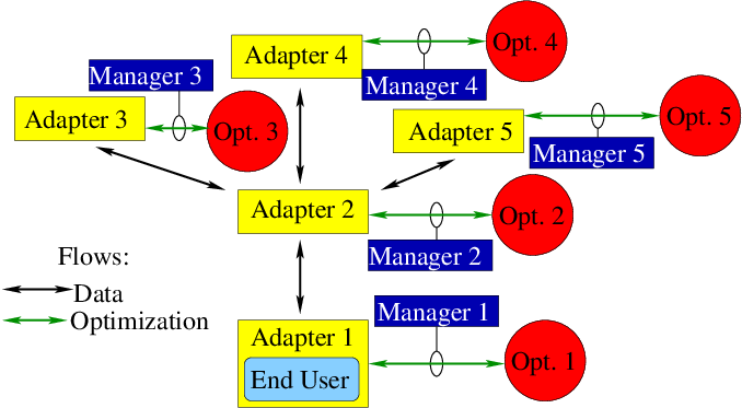
3.3.10. Solver Architecture

3.3.10.1. Input Problem Representation

Any optimization problem (including internally generated) is represented within GTOpt stack in terms of special adapters, which provide the following functionality:

• Easy and transparent problem transformation into various equivalent forms (for example, introduction of slack variables).
• Automatic problem rescaling.
• Conversion into various auxiliary sub-problems (for example, feasibility restoration).
• Easy and straightforward parallelization of problem treatment.

Then every specific optimization algorithm is to be paired with particular adapter instance.

3.3.10.2. Adapter to Optimizer Pairing

Each adapter fully specifies served optimization problem:

• Problem type (UNLP, NLP, CSP, MOP, …).
• Problem flavor (problem subtypes requiring special treatment).
• Problem kind (additional problem specific data).

Each optimizer declares its capabilities:

• Supported problem types.
• Various requirements (maximum and minimum dimension, constraints type, …).

Properties of each adapter should match those of concrete optimizer to make possible adapter to optimizer pairing. But pairing itself (among other things…) is performed by optimization manager.

3.3.10.3. Optimization Manager

Optimization manager organizes optimization flow:

• Holds database of all available optimizers:
  • Formal properties.
  • Estimated efficiency depending on formal problem properties.
  • Optimizers selection policies.
  • Other details.
• Makes the list of all suitable solvers for given input problem.
• Selects best optimizer (formal efficiency and heuristic configurable selection rules).
• Ensures the absence of dead locks in optimization tree.
• Traces actual solver efficiency, interrupts process prematurely in case of vast performance degradation.
• For bottom-level (or top-level, depending on your point of view) end-user problem invokes user’s post-processing routines.

3.3.10.4. Optimization Tree

It is important to note that potentially every optimization problem under consideration might produce several auxiliary optimization subtasks (this means that its solution requires solving additional subproblems). Within the above “blind” scheme of adapter to optimizer pairings total optimization process becomes similar to growing tree. In fact, optimization tree is “self-growing” branching tree, without any a priori given rules of growing.

For instance, branching at particular “node” (adapter-optimizer pair) depends upon:

• specific problem/algorithm assigned to this node,
• possibility to parallelize solution of this node problem, and so on.

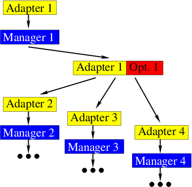
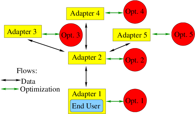
3.3.10.5. Example

Consider a simplified but logically complete example how optimization tree might look like in GTOpt. Input external problem is of the type NLP (single-objective non-linear constrained task). Depending on configurable selection policies top-level optimization manager might select the following algorithms (optimizers) to solve input problem:

• Method of multipliers (MoM).
• Sequential quadratic programming (SQP).

(We do not consider other possibilities, they are similar).

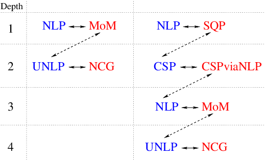
In case of MoM selection resulting optimization tree is rather simple: MoM repeatedly solves a sequence of UNLP (unconstrained non-linear) problems, each of which is passed to another instance of optimization manager. In the simplest case of NCG (non-linear conjugate gradients) selection the tree terminates: NCG produces no auxiliary subproblems, the resulting tree contains maximum two nodes. Note that this simplicity might be lost completely if manager would select QN family of methods for auxiliary UNLP: in this case another auxiliary NLP subproblem might appear due to the need to solve steepest/QN descent subtask (see section Numerical Methods for details). For simplicity we specifically assumed that manager selects NCG for UNLP problem.

Another more complex example of growing optimization tree is provided by the same input NLP task, but now selection policies dictate that SQP should be used for input problem. Sometimes SQP might enter the so called “feasibility restoration phase”, in which it tries to bring optimization process closer to feasible domain. Hence we get auxiliary CSP-type problem. Selection rules assign specific CSP solver to it, which essentially reformulates the problem as NLP and passes it further to the next instance of optimization manager (see Constraint Satisfaction Problems for details). Here a subtle point arises: manager again sees the same NLP-type problem on input, however, it must not select SQP solver because this might easily lead to an infinite loop and infinitely deep optimization tree. In our example manager selects MoM and remaining parts of optimization tree are analogous to that of previous example.