4.5. Techniques
Sections
- Gradient Boosted Regression Trees
- Gaussian Processes
- High Dimensional Approximation
- High Dimensional Approximation combined with Gaussian Processes
- Incomplete Tensor Products of Approximations
- Mixture of Approximators
- Piecewise Linear Approximation
- Response Surface Model
- Sparse Gaussian Process
- 1D Splines with tension
- Tensor Products of Approximations
- Tensored Gaussian Processes
- Table Function
4.5.1. Gradient Boosted Regression Trees
4.5.1.1. Overview
Gradient Boosted Regression Trees (GBRT) is a technique which uses decision trees as weak estimators and combines several weak estimators into a single model, in a stage-wise fashion. At each stage there is some imperfect model \(F_m\). The gradient boosting algorithm improves on it by adding a weak estimator \(h_m\) which it fits to the residual \(Y-F_m(X)\), where \(X\) and \(Y\) are true values from the training sample. The algorithm does not change \(F_m\) — instead, it produces a new model \(F_{m+1}(X) = F_m(X) + h_m(X)\), so \(F_{m+1}\) is trained to correct its predecessor \(F_m\). Each added weak estimator \(h_m\) tries to minimise the model’s mean square error over the training set (the loss function). This process is repeated until the maximum allowed number of weak estimators is reached.
GBRT algorithm has several additional parameters which are discussed in section Configuration. The algorithm is described in more detail in section Algorithm.
Advantages of the GBRT approach include:
- Relatively low training time.
- Ability to model complex functions.
- Ability to handle large data sets.
- Applicability to classification problems.
- Weighted training sample support (see Sample Weighting).
- The support for incremental model training (see Incremental Training).
Disadvantages come from the nature of weak estimators — a combination of decision trees produces a piecewise constant approximation, thus:
- Approximation is a step function (not smooth).
- Small training samples give low quality approximation.
- A GBRT model cannot be fit to training sample exactly (GTApprox/ExactFitRequired is not supported).
- GBRT models do not support smoothing and accuracy evaluation.
- GBRT models cannot calculate gradients and always return NaN as gradient values.
GBRT can approximate functions of any type. It is suitable for problems with large data sets and in cases when smooth approximation is not required.
4.5.1.2. Configuration
The GBRT technique provides several settings that control the model complexity and can act as regularization to prevent overtraining. GBRT also supports a specific usage scenario when the model is first trained using only partial data, and then can be improved by adding new training samples (see section Incremental Training for details).
4.5.1.2.1. Shrinkage
Regularization by shrinkage applies a “learning rate” to weak estimators, scaling each added weak estimator \(h_m\) by a factor \(\nu \leq 1\), so
The shrinkage step \(\nu\) is set by GTApprox/GBRTShrinkage. Typically, smaller values of GTApprox/GBRTShrinkage improve model quality, but it comes at the cost of increasing the number of weak approximators (regression trees) required to maintain low model error on the training set.
4.5.1.2.2. Stochastic Boosting
Stochastic boosting allows to train each weak estimator on a smaller subsample of the training set drawn at random. There are two subsampling options, which can be used independently or combined:
- GTApprox/GBRTSubsampleRatio randomly excludes points from the training set, so subsample size is some constant fraction of the size of the full training set.
- GTApprox/GBRTColsampleRatio randomly excludes input components (features), so the input dimension of a subsample is less than that of the full training set.
Smaller subsample sizes help prevent overtraining, acting as a kind of regularization. The algorithm also becomes faster, because regression trees have to be fit to smaller datasets at each iteration. However, stochastic boosting requires relatively low learning rate (smaller GTApprox/GBRTShrinkage values), otherwise results can be poor. Also, small subsamples require a larger number of weak estimators to obtain an accurate model.
4.5.1.2.3. Model Complexity
Overall complexity of a GBRT model can be controlled by limiting the number of boosting iterations, or the number of weak estimators in the model. Related option is GTApprox/GBRTNumberOfTrees that sets the number of regression trees to include in a model.
Another option is to set a hard limit for the complexity of weak estimators (maximum tree depth) with GTApprox/GBRTMaxDepth. Typically, increasing tree depth makes the model more accurate, but greater depth can also result in overtraining.
There is also a soft (criterion-based) limit for the complexity of weak estimators. The criterion is the loss function (model error) reduction achieved at a given tree node; if the reduction is lower than the threshold set by GTApprox/GBRTMinLossReduction, that node is not partitioned further. Note that higher threshold makes the algorithm more conservative.
4.5.1.2.4. Leaf Weighting
Variance in predictions at trees’ terminal nodes (leaves) can be reduced by limiting the allowed minimum subsample weight in a leaf. This is a natural generalization of the limit for the minimum number of points in a leaf which accounts for weights of points in the training sample if they are specified.
Related option is GTApprox/GBRTMinChildWeight. If the training sample is not weighted, all points are assumed to have a weight of 1, so GTApprox/GBRTMinChildWeight becomes simply the minimum number of points in a leaf.
4.5.1.2.5. Incremental Training
Given a GBRT model \(F_{in}\) and a new data sample, you can “update” the initial model \(F_{in}\) to obtain an improved model \(F_{up}\). Common use case is when not all data is available initially, and more samples are added progressively. Another possible scenario is the case of a huge sample which is expensive to process at once; in this case, incremental training works better with the GTApprox/MaxExpectedMemory option (see the Training with Limited Memory example).
Incremental training trains a “residual” model, which approximates differences between the response values in the new training sample and the response values calculated by the initial model \(F_{in}\) for the input values found in the new training sample. This model is added to the initial in order to better fit the data.
To perform incremental training, the initial model should be given to build() (see the initial_model argument).
By default, the “residual” model is trained with the same options as the initial model (except GTApprox/GBRTNumberOfTrees, see below).
If you change some options, your changes take priority.
Still, new settings must not select any technique except GBRT — thus all limitations of the GBRT technique also apply to incremental training.
In incremental training, GTApprox/GBRTNumberOfTrees is not affected by GTApprox/Accelerator and is not equal to the number of trees in the initial model. If GTApprox/GBRTNumberOfTrees is not set or is set to 0 (auto), the number of trees in the “residual” model is \(\max(20, N K' / K)\), where \(N\) is the total count of trees in the initial model, \(K\) is the total count of sample points used to train the initial model, and \(K'\) is the size of the new data sample (see section Algorithm for details).
When using incremental training for a model with categorical variables (see Categorical Variables), note the following:
- The GTApprox/CategoricalVariables option
must be set to the same value as the one used when training the initial model.
You can get this value from the initial model’s
details: the list of option values is stored under the"Training Options"key. - The \(\mathbf{X}\) part of the new training sample can contain new values of categorical variables (new levels). These new values will be automatically added to the list of valid values for categorical variables.
If you use an initial model trained with the output transformation feature, note that you cannot change the transformation settings that have been applied when training the initial model — see the GTApprox/OutputTransformation option description for details.
4.5.1.3. Algorithm
GBRT model \(F\) can be defined recursively as:
where \(h_m(X)\) are weak estimators, \(\nu\) is the shrinkage step, and \(M\) is the number of regression trees (or the number of gradient boosting stages).
4.5.1.3.1. Initial Training
Let \(S\) be a training sample of size \(N\) and input dimension \(d\), so \(S = (\mathbf{X}, \mathbf{Y}) = \{(X_i, Y_i), i = 1, \ldots, N\}\), where \(X_i = (x_i^{(1)}, x_i^{(2)}, \ldots, x_i^{(d)}) \in \mathbb{R}^d\) is the input part (feature values) and \(Y_i \in \mathbb{R}\) is output.
The algorithm begins with a single weak estimator \(h_1\) trained using the sample \(S\). Initial model \(F_1(X) = h_1(X)\).
Each gradient boosting stage improves the model as follows:
- Form a new training sample \(S_m\), replacing output values with residuals \(Y_i - F_{m-1}(X_i)\), so \(S_m = (\mathbf{X}, \mathbf{Y}^{(m)}) = \{(X_i, Y_i - F_{m-1}(X_i)), i = 1, \ldots, N\}\).
- Select a random subset of features (columns) from \(\mathbf{X}\), forming an input sample \(\tilde{\mathbf{X}}\) of dimension \(\alpha_c d\) (rounded up), where \(\alpha_c\) is the GTApprox/GBRTColsampleRatio value. Column subsample \(\tilde{S}_m = (\tilde{\mathbf{X}}, \mathbf{Y}^{(m)})\).
- Select a random subsample \(\hat{S}_m \subset \tilde{S}_m\) so that its size \(|\hat{S}_m| = \alpha_r |\tilde{S}_m|\) (rounded up), where \(\alpha_r\) is the GTApprox/GBRTSubsampleRatio value. \(\hat{S}_m\) is now the training sample for next weak estimator.
- Train a weak estimator \(h_m\) using the subsample \(\hat{S}_m\).
- Update the model: \(F_m(X) = F_{m-1}(X) + \nu h_m(X)\), where \(\nu\) is the GTApprox/GBRTShrinkage value (shrinkage step).
The above process is repeated until \(m\) reaches the maximum allowed number of trees set by GTApprox/GBRTNumberOfTrees. Finally, the algorithm selects a subset of points from the training sample (see Train Sample Filtering) and stores this subset into the model. The filtered subset is used when you perform incremental training (see section Incremental Training for details).
Weak estimators are also trained iteratively. GBRT uses regression trees — binary trees which partition the input domain into several cells. Each terminal node of a tree (leaf) represents a cell of the input domain, and the approximation over each cell is constant. To assign a point \(X = (x^{(1)}, x^{(2)}, \ldots, x^{(d)}) \in \mathbb{R}^d\) to a cell, the algorithm passes it down through the tree. At each node it selects a feature \(x^{(i)}\) and checks its value against a split \(\mu_i\) to move further to one of the child nodes: either where \(x^{(i)} \leq \mu_i\) or where \(x^{(i)} > \mu_i\). Both the selected feature \(x^{(i)}\) and the split value \(\mu_i\) are specific to the current node. The process is repeated until the algorithm reaches a leaf.
When growing a tree, each iteration partitions one of the existing cells of the input domain (represented by a tree leaf), beginning with the full domain on the first iteration. To partition a cell, the algorithm selects a feature \(x^{(i)}\) and finds \(\mu_i\) so as to maximize the reduction of the loss function — that is, it searches for a maximum improvement in terms of the model’s mean square error over the training set. The partitioning (in the current branch) stops if:
- the depth reaches GTApprox/GBRTMaxDepth, or
- the obtained reduction of loss is less than GTApprox/GBRTMinLossReduction (there is no significant improvement), or
- the total weight of training points assigned to a leaf is less than GTApprox/GBRTMinChildWeight.
The last criterion is a natural generalization of the limit for the number of points in a leaf which accounts for weights of points in the training sample if they are specified. If the training sample is not weighted, all points are assumed to have a weight of 1, so the weight limit becomes simply the minimum number of points in a leaf.
4.5.1.3.2. Train Sample Filtering
Each GBRT model stores a specifically selected part of the sample used to train it. This filtered sample is required in incremental training (see Incremental Training further).
Consider a training sample containing \(N\) points. Let \(S\) denote the set of indices of candidate points, and \(\bar{S}\) — the set of indices of selected points. Initially, \(S = \overline{1, N}\) and \(\bar{S} = \emptyset\) (empty). The filtering procedure \(H\) works as follows:
- Assign ranks to sample points. The rank of the \(j\)-th sample point is \(r_j = \sum\limits_{i=1}^M (\frac{1}{w_i})\). \(M\) is the number of regression trees (GTApprox/GBRTNumberOfTrees) in the model that was trained recently (in the current “residual” model, or in the initial model, if you are not performing the incremental training yet); \(w_i\) is the number of points that share the leaf with the \(j\)-th point (that is, the number of points in this leaf minus 1).
- Randomly select \(i\)-th point from the training sample with probability \(P_i = r_i / \sum\limits_{j=1}^{|S|} r_j\), where \(|S|\) is the current number of indices in \(S\).
- Add the index of the selected point \(i\) to \(\bar{S}\) so it becomes \(\bar{S} \cup \{i\}\). Discard this index from \(S\), so it is now \(S \setminus \{i\}\).
- Repeat steps 2 and 3 until \(\bar{S}\) contains \(N \cdot p\) indices (currently \(p\) is set to 0.1).
The output of the filtering procedure \(H\) is a subset of the training sample containing only those points which are indexed by \(\bar{S}\).
4.5.1.3.3. Incremental Training
Incremental training considers the situation when an initial GBRT model \(F_{in}\) already exists and the goal is to improve it using a new sample \((\mathbf{X}, \mathbf{Y})\).
The incremental training algorithm builds a “residual” model \(F_r\) that approximates the differences in responses between the new training sample and the initial model \(F_{in}\). The updated model is an ensemble of the initial and residual models: \(F_{up} = F_{in} + F_r\).
It is important that the sample actually used in incremental training is not \((\mathbf{X}, \mathbf{Y})\) alone but the union of \((\mathbf{X}, \mathbf{Y})\) and the filtered sample \((\mathbf{X}', \mathbf{Y}')\) stored with the initial model \(F_{in}\). The filtering procedure \(H\) is described above (see section Train Sample Filtering).
The algorithm works as follows:
- Create the training set as \(\breve{\mathbf{X}} = \mathbf{X}' \cup \mathbf{X}, ~~ \breve{\mathbf{Y}} = \mathbf{Y}' \cup \mathbf{Y}\).
- Calculate responses of the initial model: \(\hat{\mathbf{Y}} = F_{in}(\breve{\mathbf{X}})\).
- Calculate residuals: \(\mathbf{Z} = \breve{\mathbf{Y}} - \hat{\mathbf{Y}}\).
- Train a GBRT model \(F_r\) using \((\breve{\mathbf{X}}, \mathbf{Z})\) as the training sample.
- Add \(F_r\) to the ensemble to get the updated model: \(F_{up} = F_{in} + F_r\).
- Get an additional filtered sample: \((\bar{\mathbf{X}}, \bar{\mathbf{Y}}) = H(\mathbf{X}, \mathbf{Y})\).
- Store the updated filtered sample \((\mathbf{X}' \cup \bar{\mathbf{X}}, \mathbf{Y}' \cup \bar{\mathbf{Y}})\) with the updated model \(F_{up}\).
Note that if the number of weak estimators (regression trees) to include in \(F_r\) is not specified (GTApprox/GBRTNumberOfTrees is 0 (auto) or unset), it will not be determined by GTApprox/Accelerator (as in initial training). Instead, the number of trees will be \(\max(20, N K' / K)\), where:
- \(N\) is the total count of trees in \(F_{in}\). Total count means that if \(F_{in}\) is a result of a previous stage of incremental training, \(N\) includes all trees added on all training stages (not only the initial training stage, but all subsequent incremental training stages too).
- \(K\) is the total count of sample points used to train \(F_{in}\) (also counts all samples in incremental training).
- \(K'\) is the number of sample points in the newly added training sample \((\mathbf{X}, \mathbf{Y})\).
4.5.2. Gaussian Processes
4.5.2.1. Overview
Short name: GP
General description: A flexible non-linear, non-parametric technique for constructing of approximation by modeling training data sample as a realization of an infinite dimensional Gaussian Distribution fully defined by a mean function and a covariance function [Cressie1993], [Rasmussen2005]. Approximation is based on a posteriori mean (for the given training data) of the considered Gaussian Process with a priori selected covariance function. Acuracy Evaluation (AE) is supported and is based on the a posteriori covariance (for the given training data) of the considered Gaussian Process. GP contains the following features:
- flexible functional class for modeling covariance function (see also description of option GTApprox/GPPower below);
- an innovative algorithm of initialization of parameters of the covariance function;
- an adaptive strategy controlling the parameters of used optimization algorithm;
- an adaptive regularization algorithm for controlling the generalization ability of the approximation;
- multi-start capabilities to globalize the optimization of the parameters;
- usage of errorbars (variances of noise in output values at training points) to efficiently work with noisy problems and improve quality of approximation and AE;
- post-processing of the results to remove redundant features in the approximation.
See [Burnaev2011] for details.
Strengths and weaknesses: GP usually demonstrates accurate behavior in the case of small and medium sample sizes. Both interpolation and approximation modes are supported (interpolation mode should not be applied to noisy problems). AE is supported. GP is designed for modeling of “stationary” (spatially homogeneous) functions, therefore GP is not well-suited for modeling spatially inhomogeneous functions, functions with discontinuities etc. GP is a resource-intensive method in terms of ram capacity, therefore large samples are not supported.
Restrictions: Large dimensions are supported. Large samples are not supported.
Options:
- GTApprox/GPInteractionCardinality — allowed orders of additive covariance function (added in 1.10.3).
- GTApprox/GPLearningMode — give priority to either model accuracy or robustness (added in 1.9.6, updated in 6.15).
- GTApprox/GPMeanValue — mean of the model output mean values.
- GTApprox/GPPower — the value of p in the p-norm which is used to measure the distance between input vectors.
- GTApprox/GPTrendType — select trend type.
- GTApprox/GPType — specify the covariance function type.
4.5.2.2. Algorithm Details
Gaussian Processes (GPs) are one of the most convenient ways to define distribution on the space of functions. GP \(f(X)\) is fully determined by its mean function \(m(X) = \mathbf{E}[f(X)]\) and covariance function \(cov(f(X), f(X')) = k(X, X') = \mathbf{E}[(f(X) - m(X)) (f(X') - m(X'))]\). In the next section GP based approximation approach is described.
4.5.2.2.1. Used class of GPs
It is assumed that training data \((\mathbf{X},\mathbf{Y})\) was generated by some GP \(f(X)\)
where the noise \(\varepsilon\) is modeled by gaussian white noise with zero mean and variance \(\tilde{\sigma}^2\). GP based regression is interpolating, when it is assumed no noise, therefore interpolation regime is realized by setting \(\tilde{\sigma}^2\approx0\).
Also, it is assumed that GP \(f(X)\) has zero mean function \(m(X) = \mathbf{E}[f(X)] = 0\) and covariance function \(k(X, X')\), belonging to some parametric class of covariance functions \(k(X, X'|a)\), where \(a\) is a vector of unknown parameters. The following class of covariance functions is considered, namely squared exponential covariance function
where parameters \(a = \{\sigma, \theta_i, i = 1, \ldots, d\}\).
Under such assumptions the data sample \((\mathbf{X}, \mathbf{Y})\) is modeled by GP with zero mean and covariance function
where \(\delta(\vec{U})\) is a delta function. Thus, a posteriori (with respect to the given training sample) mean value of the process for some test point \(X^*\) takes the form
where \(\mathbf{I}\in\mathbb{R}^{|S|\times|S|}\) is an identity matrix, \(k^* = k(X^*, \mathbf{X}) = \bigl[k(X^*, X_j), j = 1, \dots, N\bigr]\), \(K = K(\mathbf{X}, \mathbf{X}) = \bigl[k(X_i, X_j), i, j = 1, \dots, N\bigr]\). This a posteriori mean value is used for prediction.
A posteriori (with respect to the given training sample) variance function for some test point \(X^*\) takes the form
This a posteriori variance is used as an accuracy evaluation of the prediction, given by a posteriori mean value.
When processing the real data, parameters of covariance function \(a\) are not known, so special tuning algorithm, described in the next section, was elaborated for their estimation.
4.5.2.2.2. Tuning of covariance function parameters
Values of covariance function parameters \(a\) are estimated using the training sample by maximizing the logarithm of corresponding likelihood, which takes the form [Burnaev2011] , [Panov2011] :
where \(|K + \tilde{\sigma}^2 \mathbf{I}|\) is a determinant of the matrix \(K + \tilde{\sigma}^2 \mathbf{I}\). Besides parameters \(a\) of covariance function noise variance \(\tilde{\sigma}^2\) is estimated as well by the solution of the following optimization problem
4.5.3. High Dimensional Approximation
4.5.3.1. Overview
Short name: HDA
General description: A non-linear, self-organizing technique for construction of approximation using linear decomposition in functions from functional dictionary consisting of both linear and nonlinear base functions. Particular example of such decomposition is so-called two-layer perceptron with nonlinear (sigmoid) activation function. HDA contains the following features:
- an advanced algorithm of division of the training set into the proper training and validating parts;
- different types of base functions, including sigmoid and Gaussian functions (see also description of options GTApprox/HDAFDLinear, GTApprox/HDAFDSigmoid and GTApprox/HDAFDGauss below);
- adaptive selection of the type and number of base functions and approximation’s complexity (see also description of options GTApprox/HDAPMin and GTApprox/HDAPMax below);
- an innovative algorithm of initialization of base functions’ parameters;
- several different optimization algorithms used to adjust the parameters, including RPROP, Levenberg-Marquardt and their modifications;
- an adaptive strategy controlling the type and parameters of used optimization algorithms;
- an adaptive regularization algorithm for controlling the generalization ability of the approximation;
- multi-start capabilities to globalize the optimization of the parameters (see also description of options GTApprox/HDAMultiMin and GTApprox/HDAMultiMax below);
- an advanced algorithm for boosting used for construction of ensembles for additional improvement of accuracy and stability (see also description of the option GTApprox/HDAPhaseCount below);
- post-processing of the results to remove redundant features in the approximation.
Strengths and weaknesses: HDA is a flexible nonlinear approximation technique, with a wide applicability in terms of space dimensions. HDA can be used with large training sets (more than 1000 points). However, HDA is not well-suited for the case of very small sample sizes. Significant training time is often necessary to obtain accurate approximation for large training samples. HDA can be applied to noisy data (see Section Noisy Problems). Usually, accuracy of HDA approximations improves as more training data are supplied. Restrictions: Interpolation mode is not supported, AE is not supported. Large samples and dimensions are supported.
Options:
- GTApprox/HDAFDGauss — include Gaussian functions into functional dictionary used in construction of approximations.
- GTApprox/HDAFDLinear — include linear functions into functional dictionary used in construction of approximations.
- GTApprox/HDAFDSigmoid — include sigmoid functions into functional dictionary used in construction of approximations.
- GTApprox/HDAHessianReduction — maximum proportion of data used in evaluating Hessian matrix.
- GTApprox/HDAMultiMax — maximum number of basic approximators constructed during one approximation phase.
- GTApprox/HDAMultiMin — minimum number of basic approximators constructed during one approximation phase.
- GTApprox/HDAPhaseCount — maximum number of approximation phases.
- GTApprox/HDAPMax — maximum allowed approximator complexity.
- GTApprox/HDAPMin — minimum allowed approximator complexity.
4.5.3.2. Algorithm description
HDA model consists of several base approximators. Each base approximator is a linear expansion in functional dictionary, i.e.
where \(\psi_i(\theta_i, X)\) is some function from the functional dictionary, parameterized by \(\theta_i\), \(p\) is the size of functional dictionary. The parameter \(p\) specifies the complexity of the approximation: the higher the value of \(p\) the more complex is the constructed model. The user can specify the minimum and maximum size of dictionary by setting GTApprox/HDAPMin and GTApprox/HDAPMax. GTApprox wil then automatically choose the optimal complexity in the specified range.
The type of functions in the dictionary is controlled by GTApprox/HDAFDLinear, GTApprox/HDAFDSigmoid and GTApprox/HDAFDGauss options and may include linear functions, sigmoid functions and Gaussian functions.
In HDA several base approximators are combined using bagging and boosting. The idea of these procedures is as follows. In bagging \(B\) approximators \(\hat{f}_1(X), \ldots, \hat{f}_B(X)\) are constructed using different subsamples of the given training sample. Then the final model is a mean of these approximators:
In boosting the approximation is constructed iteratively. In each iteration the model is defined by
where \(h_{k - 1}(X)\) corrects the errors of \((k-1)\)-th model. It means that these model approximates the difference between the outputs of given training set and prediction of \((k-1)\)-th model on the training set \(\mathbf{Y} - \hat{f}_{k - 1}(\mathbf{X})\).
In HDA model the approximators \(\hat{f}_{k - 1}\) of boosting procedure are obtained by using bagging procedure.
Both bagging and boosting increases the complexity of the final model but allows to obtain more accurate approximation. However, using large number of boosting iterations and large number of models in bagging results in increase of the training time and can lead to overfitting. More details on HDA algorithm can be found in [Belyaev2013].
The number of boosting iterations is controlled by GTApprox/HDAPhaseCount option. The number of models used in bagging is defined by GTApprox/HDAMultiMin and GTApprox/HDAMultiMax options. The optimal number of models is chosen adaptively in range specified by these options.
4.5.4. High Dimensional Approximation combined with Gaussian Processes
4.5.4.1. Overview
Short name: HDAGP
General description: HDAGP is a flexible nonlinear approximation technique, with a wide applicability in terms of space dimensions. GP usually demonstrates accurate behaviour in the case of small and medium sample sizes. However GP is mostly designed for modeling of “stationary” (spatially homogeneous) functions. HDAGP extends the ability of GP to deal with spatially inhomogeneous functions, functions with discontinuities etc. by using the HDA-based non-stationary covariance function.
Strengths and weaknesses: HDAGP usually demonstrates accurate behavior in the case of medium sample sizes. Both interpolation and approximation modes are supported (interpolation mode should not be applied to noisy problems). AE is supported. However HDAGP approximation is the slowest method compared to HDA method and GP method. HDAGP is a resource-intensive method in terms of ram capacity, therefore large samples are not supported.
Restrictions: Large dimensions are supported. Large samples are not supported.
Options: In general HDAGP algorithm contains both HDA features and GP features, therefore options of HDAGP consist of both HDA options and GP options:
HDA options:
- GTApprox/HDAFDGauss — include Gaussian functions into functional dictionary used in construction of approximations.
- GTApprox/HDAFDLinear — include linear functions into functional dictionary used in construction of approximations.
- GTApprox/HDAFDSigmoid — include sigmoid functions into functional dictionary used in construction of approximations.
- GTApprox/HDAHessianReduction — maximum proportion of data used in evaluating Hessian matrix.
- GTApprox/HDAMultiMax — maximum number of basic approximators constructed during one approximation phase.
- GTApprox/HDAMultiMin — minimum number of basic approximators constructed during one approximation phase.
- GTApprox/HDAPhaseCount — maximum number of approximation phases.
- GTApprox/HDAPMax — maximum allowed approximator complexity.
- GTApprox/HDAPMin — minimum allowed approximator complexity.
GP options:
- GTApprox/GPInteractionCardinality — allowed orders of additive covariance function (added in 1.10.3).
- GTApprox/GPLearningMode — give priority to either model accuracy or robustness (added in 1.9.6, updated in 6.15).
- GTApprox/GPMeanValue — mean of the model output mean values.
- GTApprox/GPPower — the value of p in the p-norm which is used to measure the distance between input vectors.
- GTApprox/GPTrendType — select trend type.
- GTApprox/GPType — specify the covariance function type.
4.5.4.2. Algorithm description
In short the HDAGP algorithm works as follows:
- HDA approximator is constructed and base functions from this approximator are extracted;
- Non-stationary covariance model of the data generation process is initialized by using the HDA-based non-stationary covariance function.
- Non-stationary covariance model of the data generation process is identified by maximizing likelihood of the training data.
- Post-processing of approximator’s structure is done.
See [Burnaev2011] for details.
4.5.5. Incomplete Tensor Products of Approximations
4.5.5.1. Overview
Short name: iTA
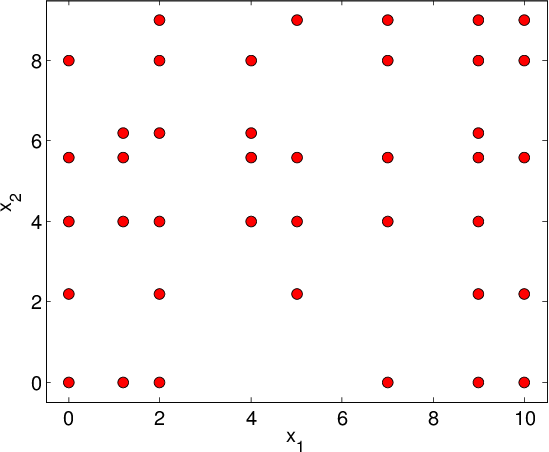
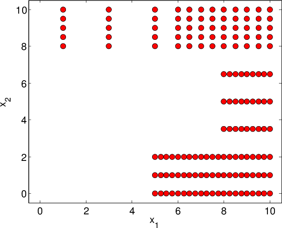
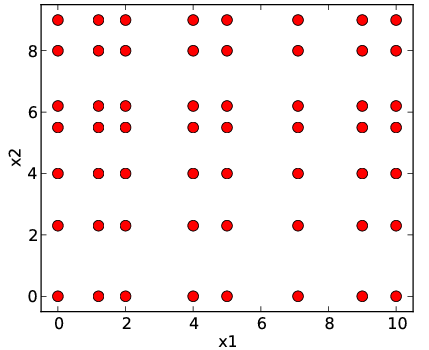
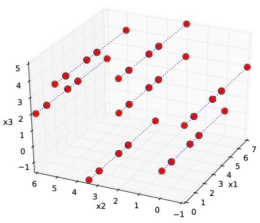
General description: Real-life designs of experiment often have a factored structure, in the sense that the DoE can be represented as a incomplete Cartesian product of two or more sets (factors). Let us denote the DoE by \(D\) and the factors by \(D_1,\ldots, D_n\); then \(D\) is a subset of the full product \(D_1\times D_2\times\ldots\times D_n\). This structure is incomplete Cartesian product. Two examples of incomplete Cartesian product are shown in Figure Examples of incomplete factored set. This type of DoE is also very common for the following reasons:
- Initial DoE was full product, but experiments are in progress (each calculation is time consuming operation).
- Some numerical solver was used for sample generation and it failed in few points (e.g. iterative process didn’t converge).
- DoE \(D\) is a union of few full factored set. Each set corresponds to typical operating conditions of the studied object (see also Figure Examples of incomplete factored set (b)).
- Incomplete grid is a special case of \(Latin hypercube\) (points are selected from the full grid).
Unlike Overview in case of incomplete grids we can’t divide the training DoE \(D\) into \(|D|/|D_k|\) “slices” since some points are missed. It’s a main reason to use explicit basis of functions instead of dictionary constructed basing on data. Such type of approximation isn’t available for multidimensional techniques implemented in GTApprox, so we can construct tensored approximation for incomplete product only if all factors \(D_k\) are one-dimensional.
Suppose that we have a tensor product of dictionaries (or basis). Now we declare this set of functions to be the dictionary for the complete approximation of \(f\), and it only remains to find a set of decomposition coefficients, like we do with the original approximation techniques. Computational complexity of this procedure depends on the type of DoE. If some points are missed then such structure get broken and this explicit formulas can’t be used. In spite of this we can reformulate problem of finding optimal coefficients as optimization problem and solve it rather efficiently (also using knowledge about data structure).
As a factorizable training DoE is a prerequisite for tensored approximations, GTApprox includes functionality to verify factorization. The user can either suggest a desired factorization to the tool or let the tool find it automatically. Also, the user can either suggest approximation techniques for individual factors or let the tool choose them automatically. These and other feature are explained in more detail in the following sections.
Mathematical details of this algorithms can be found in [Belyaev2013c] .
Strengths and weaknesses:
- It is reasonably universal: it can be used with different choices of approximation techniques in individual factors. This gives the procedure a higher degree of flexibiglity especially useful when tackling anisotropic data.
- Construction of the tensored approximation is relatively fast as its nonlinear phase only consists of nonlinear phases for individual factors (note that \(\sum_{k=1}^n |D_k|\) is typically smaller than \(|D| = \prod_{k=1}^n |D_k|\)).
- In some cases, tensored approximations have properties that are hard to achieve using generic techniques for scattered data; for example, tensored splines can provide an exact fit even for very big multi-dimensional training sets, which is not possible with standard techniques (see Section Techniques).
Restrictions: As factored data and tensored approximations have a rather special structure, they are not fully compatible with features of GTApprox developed with generic scattered data in mind. In particular, in GTApprox tensored approximations are not compatible with AE. Also, the list of approximation techniques to be tensored (see Section Approximation in single factors) is somewhat different from the list of generic techniques described in Section Techniques. Some of these restrictions are expected to be lifted in subsequent releases of GTApprox.
Options:
- GTApprox/EnableTensorFeature — enable automatic selection of TA and iTA techniques.
- GTApprox/TALinearBSPLExtrapolation — use linear extrapolation for BSPL factors (added in 1.9.4).
- GTApprox/TALinearBSPLExtrapolationRange — set linear BSPL extrapolation range (added in 1.9.4).
- GTApprox/TAModelReductionRatio — set the ratio the complexity of Tensor Approximation model should be reduced by (added in 6.2).
- GTApprox/TAReducedBSPLModel — reduce Tensor Approximation model size and memory consumption at the cost of decreased accuracy (added in 1.9.2).
- GTApprox/TensorFactors — describes tensor factors to use in the Tensor Approximation technique.
4.5.5.2. The overall workflow
The overall workflow with tensored approximations is shown in Figure The overall workflow with tensored approximations.
- Construction of tensored approximations is enabled by the option GTApprox/EnableTensorFeature. By default, GTApprox/EnableTensorFeature is \(\tt{ON}\): tensored approximations are enabled. Otherwise, if GTApprox/EnableTensorFeature is \(\tt{OFF}\), regardless of whether the training set can be factorized or not, the tool will use its generic approximation techniques and the decision tree described in Section Automatic Technique Selection, in particular disregarding the product structure if present.
Alternatively, the user can enforce tensored approximation for incomplete factorial DoE with the option GTApprox/Technique, by setting it to \(\tt{iTA}\). The main difference between these two methods is that the the usage of option GTApprox/Technique will produce an error if the factorization is not possible, while GTApprox/EnableTensorFeature set to on will create an appropriate non-tensored approximation in such case. See the decision tree The overall workflow with tensored approximations for more details.
- If tensored approximations are enabled, the tool attempts to factor the training set and to find full or incomplete product. If not successful, the tool returns to the generic techniques and decision tree (iTA technique supports one-dimensional factors only).
- Having factored the training data, the tool constructs a set of dictionaries (or basis) of functions separately for each factor, according to the approximation BSPL technique — cubic B-splines, similar to 1D Splines with tension.
4.5.5.3. Smoothing
In GTApprox, tensor products of approximations can be smoothed, and their smoothing is similar to the general smoothing described in Section Model Smoothing. Smoothing is based on penalization of second order derivatives.
4.5.5.4. Model Complexity Reduction
The complexity of the model is defined by the number of basis function used for approximation. The number of basis functions can be chosen adaptively by setting GTApprox/TAModelReductionRatio option. Note, that setting this options does not guarantee exact fit. Also this option is not compatible with GTApprox/TAReducedBSPLModel (GTApprox/TAReducedBSPLModel is deprecated since 6.2, use GTApprox/TAModelReductionRatio instead). The algorithm for selection of basis functions is the same as in TA technique. Details can be found in sectin Model Complexity Reduction.
Currently, model complexity reduction affects only BSPL factors. All other factors ignore this option.
iTA technique supports model complexity reduction since version 6.2.
4.5.6. Mixture of Approximators
4.5.6.1. Overview
Short name: MoA
General description: It is quite common situation when single approximator is not able to provide appropriate solution due to the following reasons:
- function to be approximated is spatially inhomogeneous, for example due to inhomogeneity in output design space \(\mathbf{Y}\),
- training data is inhomogeneous due to inhomogeneity in sample of input vectors \(\mathbf{X}\), or
- training sample is huge, up to million points.
The situation when function to be approximated is inhomogeneous is quite often, for example, in mechanics when computing critical buckling modes (see [Grihon2012]). For instance, function can have discontinuities and derivative-discontinuities which prevents constructing accurate surrogate model.
The case when function has a region with large gradient is shown in the Figure below. Note that this figure is given only as illustration. If training data does not have points in region with big gradient then approximation will lack accuracy in this region. However, additional sampling in domain with big gradient may not improve approximation. The surrogate model can be distorted in nearby regions: the error in the current region is decreased but the error in the neighborhood is increased.
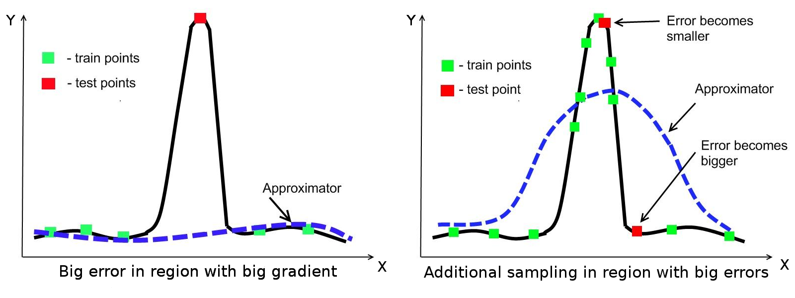
Figure: Example of function, which has a region with large gradient
When training data is inhomogeneous (for example, the set of input vectors \(\mathbf{X}\) forms some clusters in the design space) single global approximation can be not enough accurate even if function is continuous and rather smooth. For example, in case of clustered input data \(\mathbf{X}\) there is no enough data in regions between domains corresponding to clusters in \(\mathbf{X}\), that is why global nonlinear approximation can have artifacts in these regions.
Quite natural solution is to perform preliminary space partitioning and use a mixture of approximators (see [Bettebghor2011]). If the function \(F(X)\) is significantly spatially inhomogeneous, then input design space clustering is needed. So the idea is to decompose input space into domains \(\mathcal{X} = \bigcup_{j = 1}^{N_c}\mathcal{X}_j\) such that in each domain the variability of a given function is lower than in all the design space. If approximations are constructed for domains \(\mathcal{X}_j\subset\mathcal{X}\) and then are “glued”, then more accurate surrogate model can be obtained compared to the global surrogate model, constructed at once for all the design space \(\mathcal{X}\).
Strengths and weaknesses:
- MoA should be applied to inhomogeneous training data.
- Splitting training data into subsets allows to handle huge training sets. Building approximation using all the points in huge training set can be too time- and memory-consuming. Splitting training set into smaller subsets decreases time and memory consumption.
- Surrogate model in general is not represented as a single approximator, but is represented as a mixture of approximators.
Restrictions: All limitations of MoA are defined by the number of clusters and restrictions of local approximations. The general restriction on the size \(N\) of the training sample is
where \(N_c\) is the number of clusters and \(N_{min}\) is the minimal sample size required for local approximator. For example, building approximation using Gaussian Processes requires \(2d + 3\) points, where \(d\) is a dimension of input space. An error with the corresponding error code will be returned if this condition is violated. For minimal sample size, see the GTApprox user manual.
The maximum size of training sample which can be processed by the tool is primarily determined by the user’s hardware. In particular the tool was tested on huge samples up to million points, dimension up to 20 and number of clusters up to 50 on conventional PC with 4 Gb of RAM.
Options:
- GTApprox/MoACovarianceType — type of covariance matrix to use in Gaussian Mixture Model (added in 1.10.0).
- GTApprox/MoANumberOfClusters — the number of clusters (added in 1.10.0).
- GTApprox/MoAPointsAssignment — select the technique for assigning points to clusters (added in 1.10.0).
- GTApprox/MoAPointsAssignmentConfidence — confidence for points assignment technique based on Mahalanobis distance (added in 1.10.0).
- GTApprox/MoATechnique — approximation technique for local models (added in 1.10.0).
- GTApprox/MoATypeOfWeights — type of weights to use for construct final approximation (added in 1.10.0).
- GTApprox/MoAWeightsConfidence — the value to control smoothness of weights based on sigmoid function and Mahalanobis distance (added in 1.10.0).
4.5.6.2. Algorithm Details
MoA technique for construction of the surrogate model can be described as follows:
- Decomposition of the design space \(\mathcal{X}\) into connected sub-domains \(\mathcal{X}_j: \cup \mathcal{X}_j = \mathcal{X}\) corresponding to more regular behavior of the approximated dependency and/or decomposition of \(\mathbf{X}\) into more uniform parts.
- Training of local models \(g_k(X)\) using the subsamples \(S_j = \bigl\{\left(\mathbf{X}, \mathbf{Y} \right) \in S:\, \mathbf{X} \subset \mathcal{X}_j, \mathbf{Y} = F(\mathbf{X}) \bigr\}\).
- Reducing complexity by selectively excluding some sub-domains (removing some of the obtained local models). MoA excludes a sub-domain if this removal does not increase the final model’s error on the training sample. Note that on this stage it is possible that the final model will reduce to a constant, or to the initial model, if it was used (see Initial Model) — this can happen if excluding all sub-domains does not increase the model error.
- Finalizing the model by “gluing” the remaining local models.
4.5.6.3. Design Space Decomposition
In order to decompose the input design space into sub-domains in MoA currently Gaussian Mixture Model (GMM, see [Hastie2008]) is used. It is assumed that the points \((X, Y) \in S\) are generated according to the model
where \(\mu_k\) and \(\Theta_k\) are the mean vector and the covariance matrix for the \(k\)-th normal distribution of the GMM, generating sample \(S\). This model implies that design space can be decomposed into \(N_c\) homogeneous regions and in \(k\)-th region points \((X, Y)\) have gaussian distribution with parameters \(\mu_k\) and \(\Theta_k\). Parameters of the GMM are estimated using the sample \(S\) by standard EM algorithm [Hastie2008]. We should note that since for clustering not only input values were used but also output values, then possible spatial inhomogeneity of the function in the domain \(\mathcal{X}\) was taken into account. Furthermore, such model allows us to easily define distribution of the input vector \(X \in \mathcal{X}\) given \(k\)-th sub-domain:
where \(\mu_{k, x}\) and \(\Theta_{k, x}\) are the sub-vector of the mean vector \(\mu_k\) and sub-matrix of the covariance matrix \(\Theta_k\) corresponding to their \(X\)-parts.
Note that when MoA runs with an initial model \(F_{in}\) (see Initial Model), clustering is performed using the sample \(\tilde S\) which is the training sample \(S\) with outputs \(Y\) replaced by the initial model outputs \(F_{in}(X)\): \((X, F_{in}(X)) \in \tilde S\).
At that estimated parameters of the GMM in fact will provide the decomposition \(\mathcal{X} = \bigcup_{j = 1}^{N_c}\mathcal{X}_{j}\) by defining to what extent the point \(X\) “belongs” to the \(k\)-th cluster. In MoA this is done in two ways:
- By posterior probability:
(2)¶\[\mathbb{P}(k \, | \, X) = \frac{\alpha_k \mathbb{P}(X \, | \, k)} {\sum_{i = 1}^{N_c} \alpha_i \mathbb{P}(X \, | \, i)},\]where conditional probability of input vector \(X\) given \(i\)-th cluster is defined by normal Gaussian distribution with mean \(\mu_{i, x}\) and covariance \(\Theta_{i, x}\), i.e. \(\mathrm{Law}(X \, | \, i) = \mathcal{N}(\mu_{i, x}, \Theta_{i, x})\). In this case subdomain \(\mathcal{X}_k\) will consist of such points \(X\) for which posterior probability of the \(k\)-th cluster will be greater than for other clusters.
- Using Mahalanobis distance:
(3)¶\[d_k(X) = (X - \mu_{k, x})^T \left ( \Theta_{k, x} \right )^{-1} (X - \mu_{k, x})\]In this case \(\mathcal{X}_k = \left \{ X \in \mathcal{X}: \, d_k(X) \leq \chi^2_{\alpha}(d_{in}) \right \}\), where \(\chi^2_{\alpha}(p)\) is a \(\alpha\)-quantile of the distribution \(\chi^2\) with \(p\) degrees of freedom. The reason for such assignment is following. If \(X\) has Gaussian distribution with parameters \(\mu_{k, x}\) and \(\Theta_{k, x}\) then \(d_k(X)\) defined by (3) must have \(\chi^2\) distribution with \(d_{in}\) degrees of freedom. So, \(d_k(X)\) with probability \(\alpha\) must be lower than \(\chi^2_{\alpha}\). Otherwise, the point is not considered to lie in given cluster.
4.5.6.4. Calculating Model Output
The next step to obtain final approximation is to make smooth “gluing” of constructed local models. For this purpose in MoA predictions of each local model at given input vector \(X\) are calculated and the final surrogate model is defined as a weighted sum of these predictions:
where \(g_k(X)\) is a local approximation in the \(k\)-th cluster, constructed using the subsample \(S_k\), and \(w(k \, | \, X)\) are weights. In MoA weights are defined in two ways:
- By posterior probability:
(5)¶\[w(k \, | \, X) = \frac{\alpha_k \mathbb{P}(X \, | \, k)} {\sum_{i = 1}^{N_c} \alpha_i \mathbb{P}(X \, | \, i)},\]
- Based on sigmoid function:
(6)¶\[w(k \, | \, X) = \frac{1}{2} \left( \tanh \left (1 - 2 \frac{d_k(X) - \chi^2_{\alpha_0}(p)}{\chi^2_{\alpha_1}(p) - \chi^2_{\alpha_0}(p)} \right) + 1 \right ).\]Here \(\alpha_0\) coincides with confidence level used for points assignment based on Mahalanobis distance and \(\alpha_1\) controls how fast our confidence about belonging of a point to the cluster decreases with increase of Mahalanobis distance, i.e. this value sets smoothness of weights. The greater this value the smoother weights are.
Local approximations \(g_k(X)\) and weights \(w(k \, | \, X)\) are smooth functions, therefore final surrogate model (4) is a smooth function too. Each local approximator benefits into final prediction. Note, that even if local approximator has an interpolation feature the final surrogate model lacks this feature.
4.5.6.5. Initial Model
MoA can use an initial model — a previously trained model which can be improved in several ways by MoA:
- You can use the same training sample, which you used to train the initial model. In this case MoA can improve model accuracy by reducing model error on the training sample. In particular, it decomposes the design space in such a way that new sub-domains are created in the areas where the initial model has high error (see Design Space Decomposition). A new local model is then trained for each sub-domain, possibly improving accuracy.
- You can use new training data or a sample with both old and new data. In this case MoA will update the model so it fits the new data.
The initial model is added as the initial_model argument
to build().
The initial model can be trained with any technique; it is not required to be a MoA model.
The result will always be a MoA model.
When running with an initial model \(F_{in}\) and the training sample \(\left( \mathbf{X}, \mathbf{Y} \right)\), internally MoA trains a “residual” model, which approximates differences between the response values \(\mathbf{Y}\) and initial model’s outputs \(F_{in}(\mathbf{X})\). This model is then combined with the initial to better fit the data.
Option settings from the initial model do not apply to the training process in any way. If you do not set any options, the new model is trained with default settings; if you change some options, these changes apply.
If the initial model has any categorical variables (see Categorical Variables), note the following:
- The GTApprox/CategoricalVariables option
must be set to the same value as the one used when training the initial model.
You can get this value from the initial model’s
details: the list of option values is stored under the"Training Options"key. - The \(\mathbf{X}\) part of the new training sample can contain new values of categorical variables (new levels). These new values will be automatically added to the list of valid values for categorical variables.
4.5.6.6. Artificial Example: Discontinuous Function
Now let us consider two-dimensional discontinuous function:
where \(\boldsymbol{\theta}(x)\) is a Heaviside function:
Here is the figure of this function:
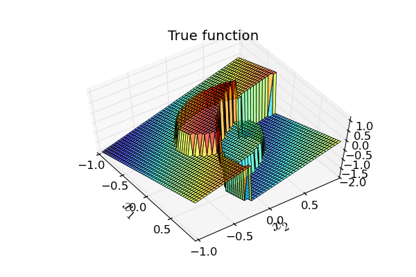
Figure: 2D discontinuous function
To construct surrogate model for this function we will use Mixture of Approximators with default parameters for local models and number of clusters in range from 2 to 10, i.e. the number of clusters was chosen automatically according to Bayesian Information Criterion. The results are depicted on Figure below.

Figure: Approximation of 2D discontinuous function
| MAE | MSE | Q95 | |
| single approx | 0.2132 | 0.3982 | 0.8188 |
| MoA | 0.1450 | 0.3172 | 0.7683 |
Approximation constructed by Mixture of Approximators is depicted on the right side of the Figure above. Different colors represent different domains into which the design space was split by the algorithm. As you can see from the picture design space has been correctly split into domains of regularity, in each domain function is quite simple to approximate. As a result we’ve obtained rather good and smooth approximation of initial function. Note that accuracy of this surrogate model is better compared to single global approximation.
4.5.7. Piecewise Linear Approximation
4.5.7.1. Overview
Short name: PLA
General description: PLA is a piecewise linear approximation based on Delaunay triangulation (for Delaunay triangulation Qhull library is used). PLA connects neighboring points of given training sample into triangles (or tetrahedra) and builds linear model in each triangle. The approximation is continuous though not smooth.
Strengths and weaknesses: PLA is a simple interpolation technique. It is suited for low-dimensional problems (1D, 2D and 3D) where the approximation is not required to be smooth. For higher dimensions the construction of surrogate model becomes computationally intractable as its complexity grows exponentially with the input dimension (complexity is \(\mathcal{O}\left ( N^{d/2}\right )\), where \(N\) is the training sample size and \(d\) is the input dimension). It is not recommended to use this technique if the data has noise.
Restrictions: Accuracy Evaluation is not supported, Smoothing is not supported.
4.5.7.2. Algorithm Details
The PLA model is a piecewise linear regression model. This technique is based on Delaunay triangulation. Triangulation is a subdivision of a given set of points into simplices, where by simplex we mean a \(d\)-dimensional tetrahedron (\(d\) is the dimension of given points).
The idea is the following. Using set of inputs \(\mathbf{X}\) we first build Delaunay Triangulation. Then in each simplex a linear regression model is constructed.
To make prediction for a new unseen point \(X^*\) the following procedure is used:
- Find in the triangulation a simplex containing the point \(X^*\). If no simplex is found the prediction at point \(X^*\) is undefined.
- Using linear model constructed for found simplex make prediction \(Y^*\) at point \(X^*\).
Note, that the linear approximation is constructed in each simplex.
Simplex has d + 1 in d-dimensional space, so the approximation passes through all the points
of the simplex exactly.
This makes the technique continuous and interpolating.
Disadvantage of such approach is that it becomes highly sensitive to the noise in the data.
It is not recommended to use this technique in case of noisy data.
PLA technique allows to make prediction only inside the constructed triangulation. If the point lies outside the convex hull of the training sample, PLA returns NaN.
PLA supports gradients for points inside triangulation. However, if point lies on the edge of a simplex PLA’s gradient is NaN. Outside the triangulation the gradients of PLA are also NaNs.
4.5.7.3. Delaunay Triangulation
Triangulation is a subdivision of the given set of points into simplices (in two-dimensional case simplex is a triangle, in three-dimensional case — tetrahedron). Each pair of simplices of triangulation should have one or less common facets. Example of triangulation is shown in figure below.
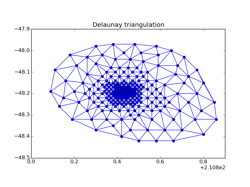
Figure: Example of Delaunay triangulation.
Delaunay triangulation is one of many triangulations that can be performed for a given set of points. It is widely used scientific computing due to its geometrical properties.
Delaunay triangulation of a set of points \(\mathbf{X}\) is a such triangulation that inside a circum-hypersphere of each simplex there are no points from set \(\mathbf{X}\).
Example of Delaunay triangulation of 4 two-dimensional points is in the figure below.
Point D is outside the circumcircle of triangle ABC and point B is outside the circumcircle of triangle ACD.
So, circumcircles are empty, they don’t contain any points inside their interior.
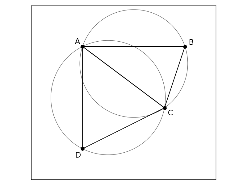
Figure: Delaunay triangulation. Circumcircles of Delaunay triangles do not contain points in their interior.
The triangulation below is different.
Circumcircle of triangle ABD contains point C.
Therefore, this triangulation is not a Delaunay triangulation.
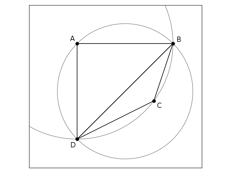
Figure: Not a Delaunay triangulation. Circumcircle of triangle ABD contains point C.
Delaunay triangles have “good shape”, because during triangulation procedure triangles with large angles are preferred to triangles with small angles. Moreover, the points are connected in nearest-neighbors manner and this additionally motivates the use of Delaunay triangulation for approximation: the closer the points, the better they can be approximated using linear function.
4.5.8. Response Surface Model
4.5.8.1. Overview
Short name: RSM
General description: RSM is a kind of linear regression model with several approaches to regression coefficients estimation. RSM can be either linear or quadratic with respect to input variables. Also RSM supports categorical input variables.
Strengths and weaknesses: A very robust and fast technique with a wide applicability in terms of the space dimensions and amount of the training data. It is, however, usually rather crude, and the approximation can hardly be significantly improved by adding new training data. In addition, the number of regression terms can increase rapidly with increasing of dimension, if quadratic RSM is used.
Restrictions: Interpolation mode is not supported, Accuracy Evaluation is not supported.
Options:
- GTApprox/RSMType — specifies the type of response surface model.
- GTApprox/RSMFeatureSelection — specifies the regularization and term selection procedures.
- GTApprox/RSMMapping — specifies mapping type for data pre-processing.
- GTApprox/RSMStepwiseFit/inmodel — selects the starting model for stepwise-fit regression.
- GTApprox/RSMStepwiseFit/penter — specifies p-value of inclusion for stepwise-fit regression.
- GTApprox/RSMStepwiseFit/premove — specifies p-value of exclusion for stepwise-fit regression.
- GTApprox/RSMCategoricalVariables — specifies categorical variables.
4.5.8.2. Description
Suppose that \(d_{out}=1\) (see Section Problem Statement). Then it is assumed that the training set is generated by the model \(\mathbf{Y} = f(\mathbf{X}) + \boldsymbol{\varepsilon}\), where
- (7)¶\[f(X) = \alpha_0 + \sum_{i = 1}^{d_{in}} \alpha_i x^{(i)} + \sum_{i, j = 1}^{d_{in}} \beta_{ij} x^{(i)} x^{(j)}, X = (x^{(1)}, \ldots, x^{(d_{in})}),\]
\(\alpha_i\) and \(\beta_{ij}\) — unknown model parameters.
\(\boldsymbol{\varepsilon}\in\mathbb{R}^{N}\) is a vector generated by white noise process.
If \(d_{out}>1\), then we construct \(d_{out}\) approximation functions \(\hat{f}_j\), \(j=1, \ldots, d_{out}\) for each component of \(Y\).
Depending on what terms in (7) are set to be zero, there are several types of RSM. Different RSM types are specified by option GTApprox/RSMType and summarized in Table.
| Type | Description |
| linear | Model contains an intercept and linear terms for each predictor (all \(\beta_{ij} = 0\)). |
| interactions | Model contains an intercept, linear terms, and all products of pairs of distinct input variables (\(\beta_{ij} = 0\) for all \(i = j\)). |
| purequadratic | Model contains an intercept, linear terms, and squared terms (\(\beta_{ij} = 0\) for all \(i \neq j\)). |
| quadratic | Model contains an intercept, linear terms, interactions, and squared terms. |
For example, in case of regularized linear regression regularization coefficient is estimated by minimization of generalized cross-validation criterion [Hastie2008]. If \(d_{out}=1\), then it is assumed that the training set is generated by the model \(\mathbf{Y} = \mathbf{X}\boldsymbol{\alpha} + \boldsymbol{\varepsilon}\), where
- \(\mathbf{Y}\in\mathbb{R}^{N}\) is a vector \((Y_1,\ldots,Y_N)\),
- \(\mathbf{X}\in\mathbb{R}^{N\times (d_{in}+1)}\) is a matrix with rows \((1, x_j^{(1)}, \ldots, x_j^{(d_{in})})\), \(j=1,\ldots,N\),
- \(\boldsymbol{\alpha}\in\mathbb{R}^{d_{in}+1}\) is a vector of unknown model parameters,
- \(\boldsymbol{\varepsilon}\in\mathbb{R}^{N}\) is a vector generated by white noise process.
4.5.8.3. Parameters Estimation
The model (7) can be written as \(f(X) = \psi(X)\boldsymbol{c}\), where \(\boldsymbol{c} = (\boldsymbol{\alpha}, \boldsymbol{\beta})\) - vector of unknown model parameters (\(\alpha_i\)‘s and \(\beta_{ij}\)‘s) and \(\psi\) - corresponding mapping. For example, \(\psi(X) = (1, \; x^{(1)}, \ldots, x^{(d_{in})}, \; x^{(1)} x^{(2)}, \; x^{(1)} x^{(3)}, \ldots, x^{(d_{in}-1)} x^{(d_{in})}, \; (x^{(1)})^2, \ldots, (x^{(d_{in})})^2)\) for the case of quadratic RSM. The output prediction for the new input \(X\) is \(\hat{Y} = \psi(X)\hat{\boldsymbol{c}}\), where \(\hat{\boldsymbol{c}}\) is an estimate of \(\boldsymbol{c}\). Let \(\mathbf{\Psi} = \psi(\mathbf{X})\) be the design matrix for the model (7).
There are a number of ways to estimate unknown coefficients \(\boldsymbol{c}\). The option GTApprox/RSMFeatureSelection specifies a particular method for estimating the coefficients:
- Least squares (GTApprox/RSMFeatureSelection = LS)
- Ridge regression (GTApprox/RSMFeatureSelection = RidgeLS)
where \(\mathbf{I}\in\mathbb{R}^{d_{in}\times d_{in}}\) and regularization coefficient \(\lambda\geq0\) is estimated by leave-one-out cross-validation [Hyman1983].
- Multiple ridge (GTApprox/RSMFeatureSelection = MultipleRidge)
where \(\mathbf{\Lambda} = diag(\lambda_1, \lambda_2, ... , \lambda_{d_{in}})\) - diagonal matrix of regularization parameters [Belyaev2011].
Regularization coefficients \(\lambda_1, \lambda_2, ... , \lambda_{d_{in}}\) are estimated successively by cross-validation. Then all the regressors, coefficients of which are greater than some threshold value, are removed from the model. We assume this threshold value to be equal to \(10^{3}\). Experiments showed that results of subset selection via multiple ridge are robust to the value of threshold.
- ElasticNet (GTApprox/RSMFeatureSelection = ElasticNet)
ElasticNet estimates coefficients \(\mathbf{c}\) by solving the following optimization problem:
i.e. ElasticNet adds to ordinary least squares optimization objective two regularization terms. The second term \(\lambda (1 - \rho) \|\mathbf{c}\|^2_2\) acts like Ridge Regression, i.e. it just shrinks coefficients towards zero. The first term \(\lambda \rho \|\mathbf{c}\|_1\) efficiently zeros out coefficients of the least important regressors (so they are actually dropped from the model). The tradeoff between them is constrolled by parameter \(\rho\) which can be set via GTApprox/RSMElasticNet/L1_ratio option. Parameter \(\lambda\) is estimated via cross-validation.
- Stepwise regression (GTApprox/RSMFeatureSelection = StepwiseFit)
Stepwise regression is ordinary least squares regression with adding and removing regressors from a model based on their statistical significance. The method begins with an initial model and then compares the explanatory power of incrementally larger and smaller models. That is, one model has \(p_1\) regressors, and the other model has \(p_2\) regressors, and \(p_1<p_2\). It is easy to see that model with \(p_2\) regressors gives lower error than model with \(p_1\) parameters. But is the larger model significantly better than the smaller model? At each step, the \(p\)-value of an \(F\)-statistic is computed to test models with and without potential regressors [Hyman1983].
The method proceeds as follows:
- Fit the initial model.
- If any regressors not in the model have \(p\)-values less than an entrance tolerance, add the one with the smallest \(p\) value and repeat this step; otherwise, go to the next step.
- If any regressors in the model have \(p\)-values greater than an exit tolerance, remove the one with the largest \(p\) value and go to the previous step; otherwise, end.
Entrance and exit tolerances are specified by options GTApprox/RSMStepwiseFit/penter and GTApprox/RSMStepwiseFit/premove accordingly.
In GTApprox two approaches for Stepwise regression are realized:
- Forward selection, which involves starting with no variables in the model, testing the addition of each variable, adding the variable that improves the model the most, and repeating this process until none improves the model.
- Backward elimination, which involves starting with all candidate variables, testing the deletion of each variable, deleting the variable that improves the model the most by being deleted, and repeating this process until no further improvement is possible.
Depending on the terms included in the initial model and the order in which terms are moved in and out, the method may build different models from the same set of potential terms.
Stepwise regression type is specified by the option GTApprox/RSMStepwiseFit/inmodel. We have GTApprox/RSMStepwiseFit/inmodel = ExcludeAll for Forward selection and GTApprox/RSMStepwiseFit/inmodel = IncludeAll for Backward elimination.
4.5.8.4. Regression Model Structure
Regression coefficients for RSM models can be obtained in an explicit form, allowing to write down the model in analytical notation.
This information is included in model details under the "Regression Model" key — see section Regression Model Information for full details.
4.5.9. Sparse Gaussian Process
4.5.9.1. Overview
Short name: SGP
General description: SGP is an approximation of GP which allows to construct GP models for larger train sets than the standard GP is able to. The motivation for SGP is both to provide a higher accuracy of the approximation and enable Accuracy Evaluation for larger training sets. Current implementation of the algorithm is based on the Nystrom approximation [Rasmussen2005] and V-technique for subset of regressors method [Foster2009].
Algorithms properties: SGP provides both approximation and AE for large training set sizes (by default, SGP is used for \(|S|\) from \(1001\) to \(9999\) if AE is required). All GP features, except interpolation, are supported.
In short, the algorithm of SGP works as follows:
- Choose a subset \(S'\) (base points) from the training set \(S\). The size of \(S'\) is \(1000\) by default, but can be changed by user.
- Initialize parameters of the SGP covariance function as parameters of GP trained with \(S'\).
- Calculate the posterior parameters of SGP.
Strengths and weaknesses: SGP can be used in case of large data sets. AE is supported. SGP is designed for modeling of “stationary” (spatially homogeneous) functions, therefore SGP is not well-suited for modeling spatially inhomogeneous functions, functions with discontinuities etc.
Restrictions: Large training sets are supported. Large dimensions are supported. Interpolation is not supported.
Options:
General GP options:
- GTApprox/GPInteractionCardinality — allowed orders of additive covariance function (added in 1.10.3).
- GTApprox/GPLearningMode — give priority to either model accuracy or robustness (added in 1.9.6).
- GTApprox/GPLinearTrend — deprecated, kept for compatibility.
- GTApprox/GPMeanValue — mean of the model output mean values.
- GTApprox/GPPower — the value of p in the p-norm which is used to measure the distance between input vectors.
- GTApprox/GPTrendType — select trend type.
- GTApprox/GPType — specify the covariance function type.
SGP specific options:
- GTApprox/SGPNumberOfBasePoints — number of the base points used to approximate the full covariance matrix of the points from the training sample.
4.5.10. 1D Splines with tension
4.5.10.1. Overview
Short name: SPLT
General description: A one-dimensional spline-based technique intended to combine the robustness of linear splines with the smoothness of cubic splines. A non-linear algorithm is used for an adaptive selection of the optimal weights on each interval between neighboring points of DoE. The default implementation in GTApprox is already interpolating, so that the GTApprox/ExactFitRequired) switch has no effect on it. See [Hyman1983], [Renka1987], [Rentrop1980] for details.
Strengths and weaknesses: A very fast technique, combining robustness of linear splines with the accuracy and smoothness of cubic splines. Interpolating. Should not be applied to very noisy problems (see Figure Different approximation techniques on a noisy problem). On the other hand, performs well if the training data is noiseless, see Figure below). Is the default method for 1D problems in GTApprox.
Restrictions: Only for 1D models (\(d_{\rm in}=1\)). Can be used with very large training sets (more than 10000 points).
Options:
- GTApprox/SPLTContinuity — required approximation smoothness.
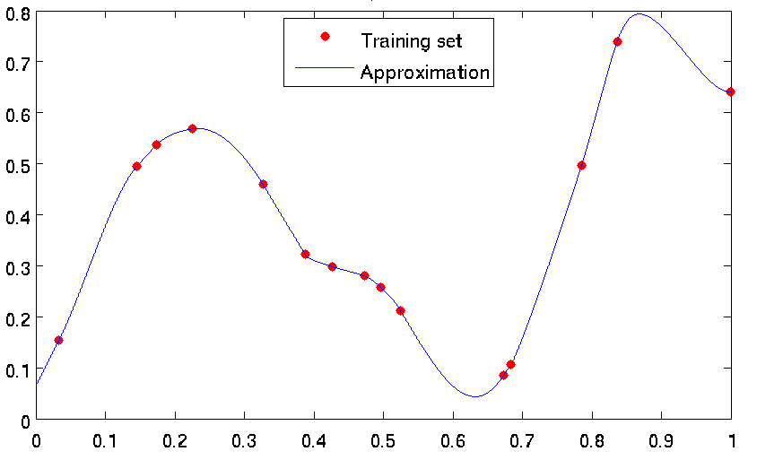
Figure: Examples of approximations constructed by GTApprox: \(d_{in} = 1, d_{out} = 1, |S| = 15\).
Note
This image was obtained using an older pSeven Core version. Actual results in the current version may differ.
4.5.11. Tensor Products of Approximations
4.5.11.1. Overview
Short name: TA
General description: Real-life designs of experiment often have a factored structure, in the sense that the DoE can be represented as a Cartesian product of two or more sets (factors). Let us denote the DoE by \(D\) and the factors by \(D_1,\ldots, D_n\); then we write the factorization as
Each factor \(D_k\) corresponds to a subset \(P_k\) of the set \(P\) of input variables \(x^{(1)},\ldots,x^{(d_{in})}\), so that to the factorization corresponds a \(partition\)
where by \(\sqcup\) we denote the union of non-intersecting sets. We refer to the number of variables in the set \(P_k\) as the \(dimension\) \(d_{in, k}\) of the corresponding factor.
These concepts are illustrated in Figure Examples of full factorizations for the case of two factors (\(n=2\)). Further details on factorization are given in Section Factorization of the training set.
- A very common special case of factorization is the standard uniform full-factorial DoE (uniform grid). Due to the “curse of dimensionality”, such a DoE is not very useful in higher dimensions, but it is very convenient and widespread in low dimensions.
- Also, in applications related to engineering or involving time series, factorization often occurs naturally when the variables are divided into two groups: one, \(P_1\), describes spatial or temporal locations of multiple measurements performed during a single experiment (for example, spatial distribution or time evolution of some physical quantity), while another group of variables, \(P_2\), corresponds to external conditions or parameters of the experiment. Typically, these two groups of variables are independent of each other: in all the experiments measurements are performed at the same locations. Moreover, there is often a significant anisotropy of the DoE with respect to this partition: each experiment is expensive (literally or figuratively), but once the experiment is performed, the values of the monitored quantity can be read off of multiple locations relatively easily — hence \(|D_1|\) is much larger than \(|D_2|\).
The general guidelines for the choice of DoE are intended for generic scattered data and clearly do not apply in the above practically important and broad class of examples (or other cases of factorization), especially in the presence of anisotropy. This motivates the special treatment of the factored DoE that we describe in this chapter.
A very natural approach to approximations on a factored DoE is based on the tensor products of approximations constructed for individual factors. The idea of this construction for the case of full factorial DoE can be explained as follows.
First note that, thanks to factorization, for each factor \(D_k\) we can divide the training DoE \(D\) into \(|D|/|D_k|\) slices of the form \(D_k\times c\), where \(c\) is an element of the complementary product \(\times_{l:l\ne k} D_l\). We can then give an alternative interpretation for the function \(f\) defined on \(D\): namely, we can view it as a function on \(D_k\) that has multiple output components indexed by \(c\in\times_{l:l\ne k} D_l\). This allows us to approximate \(f\) separately for each \(c\) using \(d_{in, k}\)-dimensional techniques. However, the drawback of this approach is that the resulting approximation is only a “partial” approximation; it is not applicable if the input variables corresponding to the factors \(\times_{l:l\ne k} D_l\) have values \(c\) other than those contained in \(\times_{l:l\ne k} D_l\).
The remedy for that is the tensor product of approximations over different \(k\). For many approximation techniques, and in particular most techniques of GTApprox, the training process includes a fast linear phase where the approximation is expanded over dictionary (some set) of functions, and, possibly, a preceding slow nonlinear phase where the appropriate dictionary is determined. For functions with multiple output components we can either choose a common dictionary for all components or choose a separate dictionary for each component (see Output Dependency Modes). Suppose that we choose a common dictionary (componentwise approximation is disabled). Let us do this for each factor \(D_k\), and then form the tensor product of the resulting \(n\) bases, i.e. form the set of vectors \(\otimes_{k=1}^n \mathbf{v}_{k,s(k)}\), where \(\mathbf{v}_{k,s(k)}\) is an element of the \(k\)-th dictionary.
Suppose that we have a tensor product of dictionaries (or basis). Now we declare this set of functions to be the dictionary for the complete approximation of \(f\), and it only remains to find a set of decomposition coefficients, like we do with the original approximation techniques. Computational complexity of this procedure depends on the type of DoE. In case of full factorial DoE set of linear coefficients can be found using explicit formulas in very efficient way thanks to special structure of the set.
As a factorizable training DoE is a prerequisite for tensored approximations, GTApprox includes functionality to verify factorization. The user can either suggest a desired factorization to the tool or let the tool find it automatically. Also, the user can either suggest approximation techniques for individual factors or let the tool choose them automatically. These and other feature are explained in more detail in the following sections. An important topic closely related to factorization in GTApprox is the concept of discrete or categorical variables (see Section Discrete/categorical variables).
Mathematical details of this algorithm can be found in [Belyaev2013b] .
Strengths and weaknesses:
- It is reasonably universal: it can be used with different choices of approximation techniques in individual factors. This gives the procedure a higher degree of flexibiglity especially useful when tackling anisotropic data.
- Construction of the tensored approximation is relatively fast as its nonlinear phase only consists of nonlinear phases for individual factors (note that \(\sum_{k=1}^n |D_k|\) is typically smaller than \(|D| = \prod_{k=1}^n |D_k|\)).
- In some cases, tensored approximations have properties that are hard to achieve using generic techniques for scattered data; for example, tensored splines can provide an exact fit even for very big multi-dimensional training sets, which is not possible with standard techniques (see Section Techniques).
Restrictions: As factored data and tensored approximations have a rather special structure, they are not fully compatible with features of GTApprox developed with generic scattered data in mind. In particular, in GTApprox tensored approximations are not compatible with AE. Also, the list of approximation techniques to be tensored (see Section Approximation in single factors) is somewhat different from the list of generic techniques described in Section Techniques. Some of these restrictions are expected to be lifted in subsequent releases of GTApprox.
Options:
- GTApprox/EnableTensorFeature — enable automatic selection of TA and iTA techniques.
- GTApprox/TADiscreteVariables — list of discrete input variables.
- GTApprox/TALinearBSPLExtrapolation — use linear extrapolation for BSPL factors (added in 1.9.4).
- GTApprox/TALinearBSPLExtrapolationRange — set linear BSPL extrapolation range (added in 1.9.4).
- GTApprox/TAModelReductionRatio — set the ratio the complexity of Tensor Approximation model should be reduced by (added in 6.2).
- GTApprox/TAReducedBSPLModel — reduce Tensor Approximation model size and memory consumption at the cost of decreased accuracy (added in 1.9.2).
- GTApprox/TensorFactors — describes tensor factors to use in the Tensor Approximation technique.
4.5.11.2. Discrete/categorical variables
TA technique supports categorical variables if they form a factor of the DoE. In this case the tool will essentially consider the function as having several components of the output, corresponding to those values of the categorical variables that are present in the training DoE. If the constructed approximation is applied to a value of the discrete variable different from all those present in the training DoE NaN value will be returned.
For more details on categorical variables see section Categorical Variables.
A variable or a set of variables can be marked as categorical using the option GTApprox/CategoricalVariables. If the marked variables do not form a factor of DoE, an error will be raised.
Alternatively, a factor can be marked as consisting of discrete variables using the option GTApprox/TensorFactors (see Section Factorization of the training set). Note that this is appropriate from the tensor product point of view, since discreteness of variables in a factor is essentially equivalent to considering the “trivial approximation” in this factor.
4.5.11.3. The overall workflow
The overall workflow with tensored approximations is shown in Figure below.
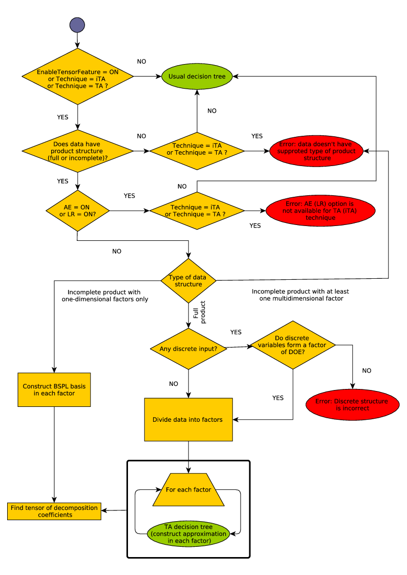
Figure: The overall workflow with tensored approximations.
- Construction of tensored approximations is enabled by the option GTApprox/EnableTensorFeature. By default, GTApprox/EnableTensorFeature is \(\tt{ON}\): tensored approximations are enabled. Otherwise, if GTApprox/EnableTensorFeature is \(\tt{OFF}\), regardless of whether the training set can be factorized or not, the tool will use its generic approximation techniques and the decision tree described in Section Automatic Technique Selection, in particular disregarding the product structure if present.
Alternatively, the user can enforce tensored approximation for full factorial DoE with the option GTApprox/Technique, by setting it to \(\tt{TA}\). The main difference between these two methods is that the the usage of option GTApprox/Technique will produce an error if the factorization is not possible, while GTApprox/EnableTensorFeature set to on will create an appropriate non-tensored approximation in such case. See the decision tree The overall workflow with tensored approximations for more details.
- If tensored approximations are enabled, the tool attempts to factor the training set and to find full or incomplete product. If not successful, the tool returns to the generic techniques and decision tree. Factorization can be either performed automatically or specified by the user through the option GTApprox/TensorFactors. See Section Factorization of the training set for more details.
- Having factored the training data, the tool constructs a set of dictionaries (or basis) of functions separately for each factor, according to the approximation technique chosen for this factor. These techniques can be either chosen automatically or specified by the user through the option GTApprox/TensorFactors. See Section Approximation in single factors for more details.
4.5.11.4. Factorization of the training set
In this section we explain in more detail our concept of factorization and how it is handled by the tool. The details of automatic factorization algorithm found below are related only to the case of a full factorial DoE and the TA technique usage.
From now on we suppose that all the input variables have a fixed order: \(x^{(1)},\ldots,x^{(d_{in})}\). Normally, this order corresponds to the positions of the variables in the input datafile.
In general, the tool supports arbitrary partitions (9) with non-empty sets \(P_k\), in the sense that if the training DoE admits factorization (8) with such a partition, then the tool can construct a corresponding TA approximation, provided an approximation can be constructed for each factor.
The user can directly specify a partition with the option GTApprox/TensorFactors. The tool will check if the partition suggested by the user is valid, i.e., the data can be factored according to it.
If the user did not specify a partition with the option GTApprox/TensorFactors, but tensoring is enabled by the option GTApprox/EnableTensorFeature, then the tool attempts to automatically find a factorization. In general, there may exist several different factorizations. For example, if a DoE of 3 variables is completely factored as \(D_1\times D_2\times D_3\), then there also are coarser factorizations obtained by grouping together some of the factors, e.g. the factorization \(D_1\times D_2'\), where \(D_2' = D_2\times D_3\). In this case we say that the first factorization is finer. If there are two different factorizations for the given DoE, then it is not hard to see that there exists a factorization which is at least as fine as either of them. As a result, for any DoE there exists a unique finest factorization (which may of course be trivial, i.e., have only one factor). Unfortunately, the exhaustive search for possible factorizations is computationally prohibitive, as the complexity of considering all partitions grows exponentially for large \(d_{in}\). For this reason, the tool performs only a restricted search, which is however sufficient for typical practical purposes. We mention two main elements of the search algorithm:
- The tool attempts to factor out all subsets of a given size if their total number (determined by the dimension \(d_{in}\)) is below some threshold value. In particular, the tool is likely to find all low-dimensional factors for moderate values of \(d_{in}\), regardless of their position among the variables \(x^{(1)},\ldots,x^{(d_{in})}\).
- In addition, the tool seeks the finest factorization within \(consecutive\) partitions. We call a partition \(consecutive\) if each of its subsets consists of consecutive variables:
for a sequence \(m_1<m_2<\ldots<m_{n-1}\). In contrast to the exponential complexity of the full search, the search over consecutive partitions is only linear in \(d_{in}\).
4.5.11.5. Approximation in single factors
In GTApprox, the following approximation techniques are available for single factors of TA technique:
- LR0 — approximation by constant
- LR — Linear Regression; deprecated option, in fact uses Response Surface Model
- BSPL — cubic B-splines, similar to SPLT of section 1D Splines with tension; only for one-dimensional factors
- GP — Gaussian Processes; as in section Gaussian Processes
- SGP — Sparse Gaussian Processes (added in 6.2); as in section Sparse Gaussian Process. The number of base points is specified by GTApprox/SGPNumberOfBasePoints. Note, that it is the same for all SGP factors. If factor size is less than the number of base points than GP technique is used for this factor.
- HDA — High Dimensional Approximation; as in section High Dimensional Approximation, but with different settings
- DV — Discrete Variables; see section Discrete/categorical variables.
Approximation techniques in TA may be either specified directly by the user or chosen automatically by the tool.
- Direct specification: If the user specifies the partition through the option GTApprox/TensorFactors, then the desired techniques may be additionally indicated for some of the factors (in the same option).
- Automatic selection: If for some factor the technique is not specified by the user, then it is determined automatically using the decision tree in Figure Decision tree for choosing approximation technique. In this decision tree, \(d_{in}\) refers to the dimension of this factor (i.e., this is \(d_{in, k}\) in the notation of Section Overview), and \(|S|\) refers to the size of DoE in this factor (i.e., this is \(|D_k|\) in the notation of Section Overview).

Figure: Decision tree for choosing approximation technique in a single factor.
4.5.11.6. Smoothing
In GTApprox, tensor products of approximations can be smoothed, and their smoothing is similar to the general smoothing described in Section Model Smoothing:
- Factors with the High Dimensional Approximation, Gaussian Processes, Sparse Gaussian Process and Response Surface Model techniques are smoothed in the usual way.
- Factors with the BSPL technique is smoothed in the same way as factors with High Dimensional Approximation technique. Smoothing is based on penalization of second order derivatives (see also section Model Smoothing).
4.5.11.7. Model Complexity Reduction
TA model can be extremely complex. For example, if all the factors are one-dimensional and BSPL techniques is used in each factor (default behavior for one-dimensional factors) the number of basis functions used to build approximation is greater than sample size (the exact number of basis functions is \(\prod_{i = 1}^n (|D_i| + 2)\)).
The model complexity can be reduced for BSPL factors by adaptively choosing basis functions.
The idea of the adaptive choice of the basis functions for BSPL factors is the following:
- For each BSPL factor choose reduced number of knots.
- In each BSPL factor place 6 knots beyond the range of the factor, other knots place according to quantiles of points in the corresponding factor. These additional 6 knots are needed to eliminate oscillations at the boundary of the range of the factor.
Number of knots is chosen to be proportional to the variability of the model with respect to the factor, i.e. if the model behavior in the factor is complex, the number of knots is large, if the behavior of the model in the factor is simple, the number of knots is small. Note, that the number of knots cannot be less than 7 (1 internal knot and 6 additional knots at the boundary). For cubic B-splines it means that we require at least 3 basis functions to be used in the factor. Therefore, the minimal model complexity has a lower bound.
Such adaptive basis function selection decreases model complexity but can result in worse approximation quality.
This functionality can be enabled by setting GTApprox/TAModelReductionRatio.
This options sets how much the complexity of the full model should be reduced.
For example, setting GTApprox/TAModelReductionRatio = 2 means that the final model should have 2 times less basis functions
compared to the default model.
Setting this option does not change saved model size. Moreover, it slightly increments model size. However, it reduces memory consumption and size of the model exported to C or Octave.
Note, that the model complexity has a lower bound. This means that the reduction ratio has an upper bound.
So, the actual reduction ration can be smaller that the value of GTApprox/TAModelReductionRatio.
Setting GTApprox/TAModelReductionRatio greater than 1 does not guarantee exact fit,
so this options is not compatible with GTApprox/ExactFitRequired set to True.
Note, that this option is not compatible with GTApprox/TAReducedBSPLModel, because both options reduce model complexity but use different algorithm to do this. GTApprox/TAModelReductionRatio is more advanced as it allows to control the complexity of the final model.
Currently, model complexity reduction affects only BSPL factors. All other factors ignore this option.
TA technique supports model complexity reduction since version 6.2.
4.5.11.8. Examples
In Figure Examples of different tensored approximations we show several different tensored approximations constructed for the same training data. In this example there are two one-dimensional factors, and the default approximation with splines in both factors looks the best. Tensored approximations with splines are usually relatively accurate and fast to construct even for large datasets; that’s why they are preferred for 1D factors. For higher-dimensional factors, however, one has to use other methods, in agreement with the decision tree in Figure Decision tree for choosing approximation technique. As usual, the choice of the approximation type in each factor primarily depends on the amount of available data: for scarce data methods with a lower flexibility, such as Response Surface Model or even LR0, are more appropriate, while for abundant data the non-linear techniques High Dimensional Approximation and Gaussian Processes are more promising.
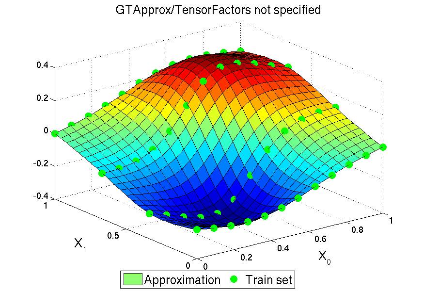
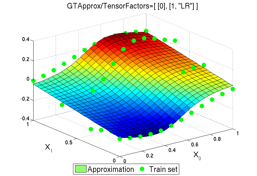
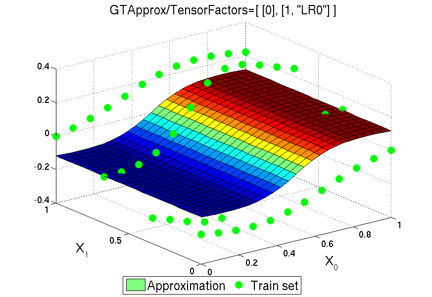
4.5.12. Tensored Gaussian Processes
4.5.12.1. Overview
Short name: TGP
General description: TGP is a powerfull technique which combines flexibility of GP model and low computational complexity of TA model. As the TA technique the TGP model can be constructed only in case of factorial DoE. In fact the TGP model is a GP model sharing all its properties. The motivation of TGP technique is high computational complexity of GP technique for large data sets which is the case for factorial DoE. However, due to the special structure of factorial DoE the compelxity of TGP technique is much more lower.
Strengths and weaknesses: TGP is in fact a GP model for training sets with factorial DoE. Therefore all GP features are supported. TGP technique has the same strengths and weaknesses as the GP technique, except computational complexity (though only factorial DoE can be used).
Restrictions: Large training sets are supported. Large dimensions are supported. Training set must have factorial DoE. Interpolation is not supported.
Options:
- GTApprox/GPLearningMode — give priority to either model accuracy or robustness (added in 1.9.6).
- GTApprox/GPLinearTrend — deprecated, kept for compatibility.
- GTApprox/GPMeanValue — mean of the model output mean values.
- GTApprox/GPPower — the value of p in the p-norm which is used to measure the distance between input vectors.
- GTApprox/GPTrendType — select trend type.
- GTApprox/GPType — specify the covariance function type.
- GTApprox/TensorFactors — describes tensor factors to use in the Tensor Approximation technique.
4.5.13. Table Function
4.5.13.1. Overview
Short name: TBL
General description: TBL is a simple table function. It tries to find input point in a predefined table of input-output pairs. If the table contains the inputs point, the model returns the corresponding output value, otherwise it returns NaN.
Strengths and weaknesses: TBL is a simple and computationally efficient technique, but it can be used only if all input variables are categorical.
Restrictions: All input variables must be categorical. Accuracy Evaluation, linearity, and model gradients are not supported.