12.7. GTDR

12.7.1. Airfoil Compression and Generation

This example consists of two parts:

• The first shows how the reconstruction error of the dimension reduction procedure may vary depending on the model (reduced) dimension.
• The second illustrates a specific case of dimension reduction model usage (airfoil generation).

To train the GTDR model in this example, we use the sample with real airfoil definitions. This is a very important point in building dimension reduction models: the training data used determines the model behavior and thus should be valid — else the model behavior will be unpredictable.

The training sample (airfoils.csv) was obtained by processing a test dataset (coord_seligFmt.zip) from the open UIUC Airfoil Coordinates Database. Describing the details of the processing procedure is beyond the scope of explanations for this example — in general, it is an airfoil coordinate conversion involving cubic polynomial spline interpolations which is required to unify the airfoil descriptions found in the test dataset. The result of such conversion is an airfoil described by a 59-dimensional vector of y-coordinates of the contour points:

\[\mathbf{\overline x} = (x_1, x_2, \dots, x_N), N = 59\]

The x-coordinates are given by a fixed x-mesh, so the airfoil may be plotted as follows:

It is also worth noting that:

1. The description always includes the contour point at \((0, 0)\) (point K). In fact this is redundant data, and GTDR will detect it, reporting that effective input dimension is 58 (this warning will be seen in the model build log).
2. Trailing edge is considered to be smooth, so the airfoil description does not include the trailing edge point. Also, the first and the last point are always symmetric with respect to the X-axis.

The airfoils.csv file contains 199 airfoils in the format described above. Each airfoil is a CSV row, contour point coordinates are separated by commas.

An additional sample afl_test.csv contains the x-mesh (first row) and a reference airfoil (second row) which we will use to test the reconstruction error.

For the first part of the example, we will construct several dimension reduction models for different reduced dimensions and show how the reconstitution error changes using GTDR internal model info. We also illustrate this by compressing and decompressing the same input vector (the reference airfoil) with each model and plotting the reconstructed airfoils vs the original reference airfoil.

For the second part, we will arbitrarily choose one of the models built before, generate a few random vectors in the compressed space (random compressed airfoils), decompress and plot them. The key point here is that due to the re-parameterization which is the result of dimension reduction, random generation in the compressed design space will likely yield a valid airfoil, contrary to the random generation in the original design space. This is one of the basic methods used in airfoil design optimization.

Begin with importing modules. Note that this example requires Matplotlib for plotting; it is recommended to use at least version 1.1 to render the plots correctly.

from da.p7core import gtdr
from da.p7core import loggers

import numpy as np
import matplotlib.pyplot as plt

import os

Define the method to build dimension reduction models for various dimensions (reduced_dimensions list). Compression/decompression error (rec_error) for each model will be output to the console after the model build log:

def build_models(data, reduced_dimensions):
  """
  Build GTDR models for various reduced (target) dimensions using
  dimension-based DR. All GTDR options are left default.
  """
  # Create GTDR model builder:
  builder = gtdr.Builder()
  # Create logger and connect it to builder:
  logger = loggers.StreamLogger()
  builder.set_logger(logger)
  # Build models:
  models = []
  for dim in reduced_dimensions:
    print('=' * 79)
    print('Building GTDR model for target dimension %d...' % (dim))
    print('=' * 79)
    model = builder.build(x = data, dim = dim)
    print('=' * 79)
    # Check the reduced dimension for the model just built:
    print('Reduced dimension: %d' % (model.compressed_dim))
    # Check the reconstruction error value:
    rec_error = model.info['DimensionReduction'] \
                          ['Training Set Accuracy'] \
                          ['Compression/decompression error (L2-norm)']
    print('Average reconstruction error: %s' % (rec_error))
    print('=' * 79)
    models.append(model)

  return models

Next, the method to reconstruct a reference airfoil (ref_airfoil) with different models built by build_models() above:

def reconstruct_airfoils(models, ref_airfoil):
  """
  Apply compression/decompression to the reference airfoil
  using GTDR models with different reduced dimensions.

  Returns a list of tuples (dimension, airfoil).
  """
  reconstructed_airfoils = []
  for m in models:
    # Get reduced dimension from model info:
    dim = m.compressed_dim
    # Reconstruct (compress and decompress) an airfoil:
    reconstructed = m.decompress(m.compress(ref_airfoil))
    reconstructed_airfoils.append((dim, reconstructed))

  return reconstructed_airfoils

To generate new airfoils, we will have to define compressed design space bounds somehow. Here we simply compress a reference data sample with the selected model (actually it will be the same sample which was used in model training; see the main() function definition), determine its bounding box, then select an area inside this box by reducing its size arbitrarily. Note that it is a simplified method which we use for example purposes only.

def generate_airfoils(num, model, ref_data):
  """
  Generate airfoils by taking a random vector in the compressed design space
  and decompressing it to the original dimension using the given GTDR model.

  This implementation is very crude: compressed vector generation algorithm
  drastically affects the quality of results, and straightforward
  randomization, like the one in this method, in fact produces low-quality
  results.

  Despite this, the probability of generating a correct airfoil with this
  method is high enough.
  """
  # Compress the reference data sample to determine the box bounds
  # in the compressed design space:
  comp_data = model.compress(ref_data)
  comp_dim = model.compressed_dim
  # All vectors from the reference sample, when compressed, are bound
  # to this box:
  x_min = np.min(comp_data, axis=0)
  x_max = np.max(comp_data, axis=0)
  # We will shrink the compressed design space a bit to exclude worst points
  # (points which are too close to the box bounds):
  shrink_by = 0.15
  x_min *= 1 - shrink_by
  x_max *= 1 - shrink_by

  # Generate:
  generated_airfoils = []
  for _ in range(num):
    # Random vector in the compressed space bound to (x_min, x_max):
    rnd_afl = np.multiply(np.random.rand(comp_dim), x_max - x_min) + x_min
    # Decompress it to get an airfoil in original design space:
    rnd_afl = model.decompress(rnd_afl)
    generated_airfoils.append(rnd_afl)

  return generated_airfoils

We did not fix the random generator seed, so generated airfoils will be different in each script run. This generation does not guarantee a valid result, though dramatically increases the probability of this, compared to the random generation in the original design space. Occasionally, generated airfoils may be not valid; you may re-run the example several times and compare the generation results.

Plotting method creates two subplots with reconstructed and generated airfoils and saves the plot to the directory where you have started the script:

def plot_results(mesh, ref_airfoil, rec_airfoils, gen_airfoils):
  """
  Plot the reference airfoils, reconstructed airfoils and new generated
  airfoil vs the x-mesh.
  """
  fig = plt.figure(1)
  fig.subplots_adjust(left=0.2, wspace=0.6, hspace=0.6)
  # First subplot, reference and reconstructed airfoils:
  plt.subplot(211)
  plt.plot(mesh, ref_airfoil, label = 'Reference')
  for dim, afl in rec_airfoils:
    plt.plot(mesh, afl, label = 'Dimension: %s' % (dim))
  plt.legend(loc = 'best', prop={'size':8})
  plt.title('Reconstructed Airfoils')
  # Second subplot, generated airfoils:
  plt.subplot(212)
  for afl in gen_airfoils:
    plt.plot(mesh, afl)
  plt.title('Generated Airfoils')
  # Save the plot to current working directory:
  plot_name = 'gtdr_airfoils_example'
  plt.savefig(plot_name)
  print('Plot saved to %s.png' % os.path.join(os.getcwd(), plot_name))
  # Show the plot:
  if 'SUPPRESS_SHOW_PLOTS' not in os.environ:
    print('Close the plot window to finish.')
    plt.show()

Finally, we put it all together in the main() function. This is the main workflow with the following steps:

1. Specify a list of model (reduced) dimensions. Dimensions are chosen arbitrarily, you may specify another dimensions list.
2. Locate sample files — have to be placed in the same directory with the script.
3. Load the training sample from airfoils.csv.
4. Load the x-mesh and the reference airfoil from afl_test.csv.
5. Build GTDR models for the specified dimensions by build_models().
6. Reconstruct the reference airfoil with each model by reconstruct_airfoils()
7. Select the model to use in airfoil generation and run generate_airfoils() to get some new airfoils.
8. Plot the reference airfoil, a reconstructed reference airfoil for each dimension reduction model, and the new generated airfoils.

def main():
  # Various reduced (target) dimensions for testing the reconstruction
  # accuracy of GTDR models:
  dimensions = [1, 3, 5, 7]

  # Locate resources:
  script_path = os.path.dirname(os.path.realpath(__file__))
  train_afl_path = os.path.join(script_path, 'airfoils.csv')
  ref_afl_path = os.path.join(script_path, 'afl_test.csv')

  # Load training data:
  print('=' * 79)
  print('Loading airfoil data for training...')
  print('=' * 79)
  train_airfoils = np.loadtxt(train_afl_path, delimiter=',')
  print('Original dimension: %d' % len(train_airfoils[0]))

  # Load the x-mesh (first row) and a reference airfoil (second row)
  # from a CSV file.
  print('=' * 79)
  print('Loading x-mesh and reference airfoil...')
  print('=' * 79)
  mesh, ref_airfoil = np.loadtxt(ref_afl_path, delimiter=',')

  # Build models of specified dimensions:
  print('=' * 79)
  print('Building GTDR models for target dimensions: %s' % (dimensions))
  print('=' * 79)
  models = build_models(train_airfoils, dimensions)

  # Reconstruction:
  print('=' * 79)
  print('Reconstructing the reference airfoil (dimensions: %s).' % (dimensions))
  print('=' * 79)
  reconstructed_airfoils = reconstruct_airfoils(models, ref_airfoil)

  # Generation - select the model (determines generation space dimensionality)
  # and the number of airfoils to generate:
  gen_model = models[3]
  num = 3
  dim = gen_model.compressed_dim
  print('=' * 79)
  print('Generating %s new airfoils in %s-dimensional space...' % (num, dim))
  print('=' * 79)
  gen_airfoils = generate_airfoils(num, gen_model, train_airfoils)

  # Finally, make the plots:
  plot_results(mesh, ref_airfoil, reconstructed_airfoils, gen_airfoils)

if __name__ == '__main__':
  main()

To run the example, open a command prompt and execute:

python -m da.p7core.examples.gtdr.example_gtdr_airfoil

You can also get the input sample (airfoils.csv), x-mesh and reference airfoil (afl_test.csv) and the full code (example_gtdr_airfoil.py) to run the example as a script. All three files have to be placed in the same directory.

Resulting plot for this example looks like this:

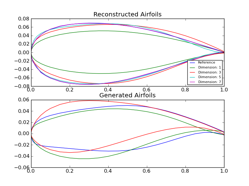
Note that the reconstructed airfoils subplot is reproducible, while the actual generated airfoils subplot will differ from the one shown, due to the random generation. We intentionally selected a result which contains an invalid generated airfoil (the one with intersection): it is a typical error of the simplified generation method used in this example.

More GTDR examples can also be found in Code Samples.