4.3. Approximation Modes¶

Sections

Exact Fit
Noisy Problems
- Heteroscedastic data
- Data with Errorbars
Output Dependency Modes
Sample Weighting
Categorical Variables
Categorical Outputs
Submodels and Parallel Training

4.3.1. Exact Fit ¶

The exact fit mode can be set by the option GTApprox/ExactFitRequired (default value is off). If this switch is turned on, then the constructed approximation will go through the points of the training sample (see Figure below). If the switch is off, then no interpolation condition is imposed, and the approximation can be either interpolating or non-interpolating depending on which fits the training data best.

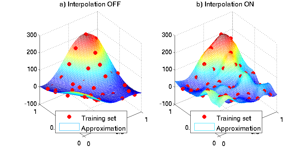
Figure: Examples of approximations constructed from the same training data with Interpolation OFF or ON.

The exact fit mode is supported only by the following techniques:

Gaussian Processes and Tensored Gaussian Processes: supported, but only if GTApprox/GPLearningMode is not set to "Robust".
Tensor Products of Approximations: supported for GP and SPLT factors only.
1D Splines with tension, Piecewise Linear Approximation, and Table Function: these techniques are always exact-fitting by definition.

All techniques which are not mentioned above do not support the exact fit mode. Also, this mode is computationally demanding and therefore is restricted to moderately sized training samples.

The following guidelines are important when choosing whether to switch the exact fit mode on or off:

If the approximation has a low error on the training sample (in particular, if it is a strict interpolation), it does not mean that this approximation will be just as accurate outside of the training sample. Very often (though not always), requiring an excessively small error on the training sample leads to an excessively complex approximation with low predictive power — a phenomenon known as overfitting or overtraining (see, e.g., [Everitt2002], [Tetko1995] ). This phenomenon consists in getting the approximation to be very accurate on the training DoE, at the cost of excessively increasing approximation’s complexity which leads to a less robust behavior and ultimately lower accuracy on points not belonging to the training set (see, e.g., [Runge1901] for the classical example of Runge’s phenomenon). The errors of an overfitted approximation on a training set are usually much lower that the errors on the independent test set. If the strict interpolation mode is off, GTApprox attempts to avoid overfitting.
The interpolation mode is inappropriate for noisy models. Also, if the training sample is highly irregular or the approximated function is known to be singular, then the interpolation mode is not recommended, as in this case the approximation tends to be numerically unstable. On the whole, strictly interpolating approximations are more flexible but less robust than non-interpolating ones.
The interpolation mode may be useful, e.g., if the default approximation (with the interpolation mode off) appears to be too crude. In this case, turning the interpolation mode on may (but is not guaranteed to; the opposite effect is also possible) increase the accuracy.

Because of numerical limitations and round-off errors, minor discrepancies can be observed in some cases between the training sets and the interpolating approximations constructed by GTApprox. These discrepancies typically have relative values \(\lesssim 10^{-5}\) and are considered negligible.

4.3.2. Noisy Problems ¶

By noisy problems one usually understands those problems where the response function is a regular function perturbed by a random, unpredictable noise. In these problems one is typically interested in some noise-filtering and smoothing of the training data so as to recover the regular dependence rather than reproduce the noise; in particular, strict interpolation is unnecessary and possibly undesirable. The extreme case of noisy problems are those with training data containing points with the same input, but different output (e.g., random variations in the results of different experiments performed under the same conditions). The sensitivity of an approximation method to the noise is usually positively correlated with the interpolating capabilities of the method and negatively correlated with its crudeness.

Table summarizes how the methods of GTApprox can be ordered with respect to their noise sensitivity, from the most sensitive to the least sensitive. The table refers to the default versions of the methods, with the interpolation mode turned off (see Section Exact Fit). User is advised to adjust the level of smoothing in particular problems by choosing the appropriate approximation technique of GTApprox.

Noise-sensitivity of different approximation techniques with default settings in **GTApprox**.¶
SPLT	Strictly interpolating, very noise-sensitive.
GP, SGP, HDAGP	Not strictly interpolating in general, tend to somewhat smoothen the data (degree of smoothing depends on a particular problem).
HDA	Mostly smoothing. Sensitivity can be further tuned by adjusting the complexity parameters of the approximation through advanced options, see HDA. Can be applied to very noisy problems with multiple outputs corresponding to the same input.
RSM	The crudest and most robust method. Very noise-insensitive.

An example of the application of different methods of GTApprox to a 1D noisy problem is shown in Figure below.

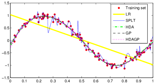
Figure: Different approximation techniques on a noisy problem.

Note

This image was obtained using an older pSeven Core version. Actual results in the current version may differ.

4.3.2.1. Heteroscedastic data ¶

It is usually assumed that the noise in output data sample has uniform properties and can be modelled by independent identically distributed multivariate normal variables (particular case of homoscedastic noise). However, in some approximation problems noise can be heteroscedastic, e.g. when output variance depends on the point location in the design space. For such problems, the noise in some regions may be negligible, while in other regions the presence of noise has to be taken into account to build an accurate enough approximation and provide consistent accuracy evaluation.

To resolve such issues, GTApprox implements a dedicated algorithm based on Gaussian processes. It assumes the following form of the output:

\[f(X) = f_1(X) + \varepsilon(X),\]

where \(f_1(X)\) is a realization of a Gaussian process, \(\varepsilon(X)\) is white noise with zero mean and variance given as \(\exp\! \left(f_2(X) \right)\) where \(f_2(X)\) is also a realization of a Gaussian process. During training we estimate parameters of Gaussian processes \(f_1(X)\) and \(f_2(X)\); \(f_1(X)\) models the true function, while \(f_2(X)\) models the noise in the output data.

Direct inference in this case isn’t possible, so approximate inference is used to adjust model parameters and estimate function value and accuracy evaluation at a new point.

The above algorithm is used only when the GTApprox/Heteroscedastic option is on. By default it is assumed that the data is homoscedastic, and heteroscedastic version of Gaussian process is not used.

Specific features of the heteroscedastic Gaussian processes are:

This algorithm is only available when Gaussian Processes or High Dimensional Approximation combined with Gaussian Processes technique is used.
Accuracy evaluation is available and typically is significantly more accurate than that of Gaussian Processes and High Dimensional Approximation combined with Gaussian Processes with Heteroscedastic option off, if the input data is really heteroscedastic.
Due to the limitations of Gaussian Processes and High Dimensional Approximation combined with Gaussian Processes techniques, their heteroscedastic versions are only useful if the sample size \(S\) does not exceed a few thousands of points.
This algorithm is not compatible with the Mahalanobis covariance function for GP and with explicit specification of the input variance (see Section Data with Errorbars).

An example result of using the heteroscedastic algorithm is shown on figure below. There, original function is one-dimensional piecewise quadratic function. It was corrupted with white noise which quadratically increases its standard deviation with larger values of input \(X\). Note how accuracy evaluation in the second case (heteroscedastic GP, right) correctly reflects the heteroscedasticity in the given data sample, compared to ordinary GP (left).

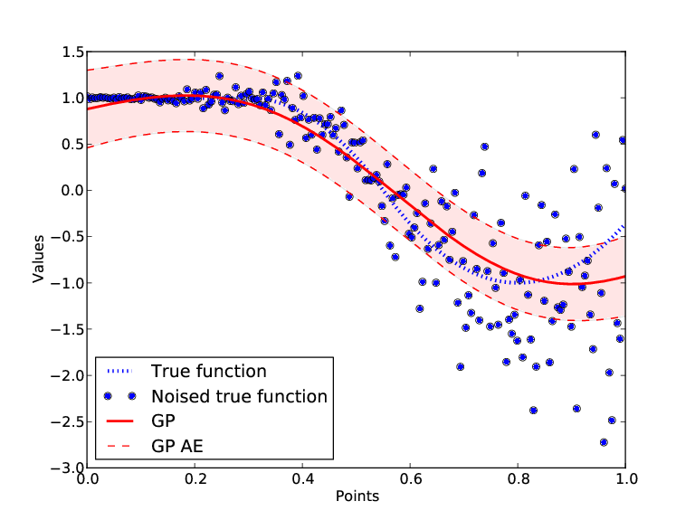
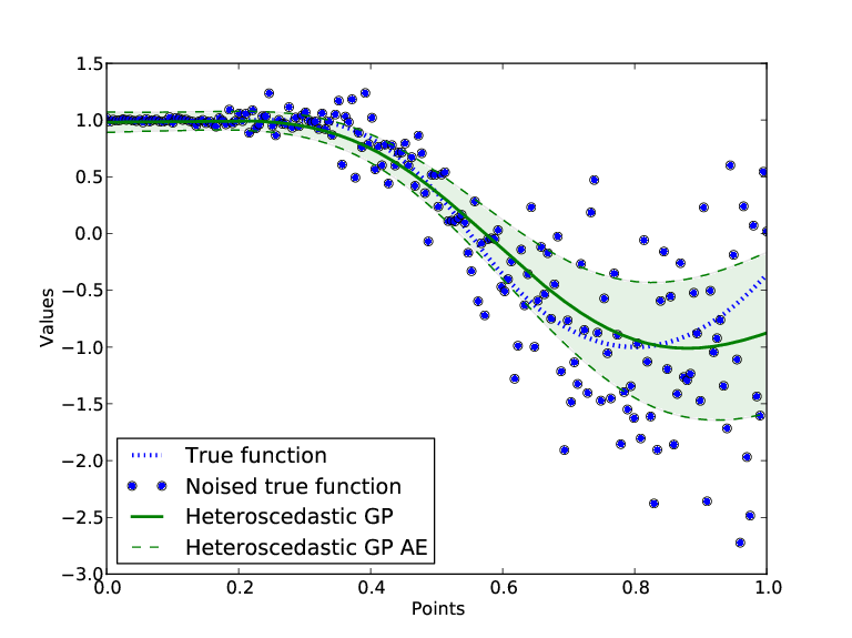
Figure: The results of GP technique, ordinary vs. heteroscedastic version.

4.3.2.2. Data with Errorbars ¶

If the user has specific knowledge about the level of noise in his data, namely variances of noise in output values at the training points, those values (errorbars) can be provided to GTApprox through the outputNoiseVariance argument to build() or build_smart(). If errorbars are set then algorithms of GTApprox will use them for additional smoothing of the model.

This functionality is supported only by the following tehcniques (others ignore outputNoiseVariance):

Depending on the type of covariance function used in GP model, usage of errorbars will have different influence on GP approximation. The best effect is expected for \(Wlp\) covariance function with \(GPPower = 2\) (See Section Gaussian Processes for details of GP options). For \(1 \leq GPower < 2\) the improvement of the model is less significant. Errorbars are especially helpful if level of noise is relatively high (5 or more percents of output function values).

4.3.3. Output Dependency Modes ¶

When the response function is multidimensional (there are \(d_{out} > 1\) responses), there are several possible approaches to training the model. GTApprox supports the following:

In the independent outputs mode (default), a separate approximator is used for each response. This mode is similar to training a separate model for each output.
In the dependent outputs mode, the same approximator is used for all output components simultaneously. This mode is not compatible with categorical outputs (see Categorical Outputs).
In the partial linear dependency mode, GTApprox tests the training sample to find linear dependencies between responses, and trains a special model which keeps these dependencies. It means that if there exists some subset of responses \(Y^{(i_1)}, ..., Y^{(i_k)}, ~ k \leq d_{out}\), such that for every measurement \(\{X_s, Y_s\}, ~ s = 1, ..., |S|\) in the training sample \(S\) holds

\[w_1 \cdot Y^{(i_1)}_s + ... + w_k \cdot Y^{(i_k)}_s = h + e_s,\]

where \(w_1, ..., w_k \in R\) are some non-zero coefficients, \(h \in R\) is some constant, which is not a priori known, and \(e_s\) is possible noise, then the model trained in the partial linear dependency mode keeps the above relation for its corresponding outputs \(\hat{f}{}^{(i_1)}, ..., \hat{f}{}^{(i_k)}\) such that

\[w_1 \cdot \hat{f}{}^{(i_1)} (X) + ... + w_k \cdot \hat{f}{}^{(i_k)} (X) = \hat{h}, ~ \forall X \in B,\]

where \(B\) is the model’s bounding box, and \(\hat{h}\) is an \(h\) estimate coming from an additional internal model of dependency between outputs.

The partial linear dependency mode is not compatible with categorical outputs (see Categorical Outputs).

Changed in version 6.3: prior to 6.3, the dependent outputs mode was default.

Changed in version 6.15: added the partial linear dependency mode.

Changed in version 6.29: added an option to specify an error threshold for the linear output dependency model.

The output dependency mode is selected using the GTApprox/DependentOutputs option.

When GTApprox/DependentOutputs is False, GTApprox assumes that output components are independent and uses componentwise approximation. Essentially it trains a separate independent submodel for each output component. When the training dataset includes multiple outputs which have significantly different behavior, independent training often results in higher model accuracy. This mode also enables efficient parallelization, since the independent submodels for output components can be trained in parallel (see Submodels and Parallel Training). However, componentwise approximation cannot consider possible dependencies between different output components — which may be the case, for example, when the outputs have the same physical meaning.

When GTApprox/DependentOutputs is True, GTApprox treats all output components as possibly dependent and does not use componentwise approximation. In cases when output dependencies do exist, a model trained in this mode is often more accurate than a model with independent outputs. Also, if parallellization is not used (submodels are trained sequentially, see Submodels and Parallel Training), training in the dependent outputs mode can be faster than in other modes.

Setting GTApprox/DependentOutputs to "PartialLinear" switches to the special “partial dependency” mode which finds dependent outputs and keeps the dependencies between them. In this mode GTApprox performs several statistical tests which are aimed to discover linear dependencies. A test passes if the training sample output data can be fitted to one of the dependency models with RRMS error that does not exceed the threshold set by GTApprox/PartialDependentOutputs/RRMSThreshold. The dependency model can be one of the following two kinds:

Explanation: dependencies of the form \(Y^{(i)} = \sum_{j=1}^{m} w_j Y^{(j)} + C\), where \(Y^{(i)}\) is the dependent output, \(Y^{(j)}, ~ j \in [1, m]\) are \(m\) explaining (independent) outputs, \(w_j\) are weight coefficients, and \(C\) is some constant. The explaining outputs are treated as independent (componentwise approximation), while the explained (dependent) output is not approximated at all.

This kind is selected if the weighted sum of variances of explaining outputs is less than the variance of the dependent output: \(\sum_{j=1}^{m} w_j^2 \mathrm{Var}(Y^{(j)}) < \mathrm{Var}(Y^{(i)})\), so the RRMS error of approximation for \(Y^{(i)}\) is not greater than RRMS errors of approximations for explaining outputs. Constant outputs and simple dependencies of the form \(Y^{(i)} = w_j Y^{(j)} + C\) also belong to this kind.
Constraint: dependencies of the form \(\sum_{j=1}^{m} w_j Y^{(j)} = C\). The outputs \(Y^{(j)}\) are approximated independently, but when the model is evaluated, it uses a special iterative algorithm which adjusts the output values to satisfy the constraint.

If it is known that outputs are linearly dependent but GTApprox cannot find that dependency, it may be caused by noisy output data in the training sample. In such cases, increasing GTApprox/PartialDependentOutputs/RRMSThreshold helps to find the dependency, as the error threshold is low by default. However, setting the threshold too high may lead to false positive dependency test results — that is, GTApprox may unexpectedly assume linear dependency between some independent outputs.

The linear dependency mode can decrease model training time if dependencies of the explanation kind are found, because there is no need to train submodels for explained outputs. However, the model may become more computationally expensive to evaluate if it contains dependencies of the constraint kind, because evaluation in this case is a three-stage process:

Evaluate independent outputs.
Iteratively adjust the independent outputs which are subject to constraints.
Calculate dependent (explained) outputs.

Finally, note that the effects described above, such as the possibility to improve model accuracy, are not guaranteed. Sometimes changing the output dependency mode has no significant effect, and it may be impossible to justify certain mode selection even with certain a priori knowledge about the data and underlying dependency.

4.3.4. Sample Weighting ¶

A number of GTApprox techniques support sample point weighting. Roughly, point weight is a relative confidence characteristic for this point which affects the model fit to the training sample. The model will try to fit the points with greater weights better, possibly at the cost of decreasing accuracy for the points with lesser weights. The points with zero weight may be completely ignored when fitting the model.

Point weighting is supported in the following techniques:

That is, to use point weights meaningfully, one of the techniques above has to be selected using GTApprox/Technique in addition to specifying weights. If any other technique is selected, either manually or automatically, weights are ignored (but see the next note).

Note

Point weighting is not compatible with GTApprox/ExactFitRequired.

Point weight is an arbitrary non-negative float value or infinity. This value has no specific meaning, it simply notes the relative “importance” of a point compared to other points in the training sample. The weights argument should be a 1D array of point weights, and its length has to be equal to the number of training sample points.

Note

At least one weight has to be non-zero.

Note

Point weighting is not compatible with output noise variance. This holds even if you select a technique that does not support output noise variance or point weighting and would normally ignore these arguments.

4.3.5. Categorical Variables ¶

Changed in version 6.25: if the training sample is a pandas.DataFrame or pandas.Series, categorical variables may be specified by sample’s dtypes instead of the GTApprox/CategoricalVariables option.

A categorical variable is a variable which can take only a limited number of values from a predefined set. These values are called levels. Categorical variables can be used to represent discrete numerical variables which are bound to a finite range, or even non-numeric variables. For example, when your data contains a string variable which has a limited number of possible values, you can encode these string values with different numbers to treat the variable as categorical.

By default, GTApprox treats all input variables as continuous. There are two general ways to specify categorical variables:

Set the GTApprox/CategoricalVariables option, which specifies indexes of categorical variables.
Pass training sample inputs as a pandas.DataFrame (pandas.Series if 1D). In this case, columns (series) with dtype categorical, string, Boolean, or object are interpreted as categorical data. Values of categorical variables in pandas.DataFrame and pandas.Series are converted to float when possible, and to strings otherwise.

For Tensor Products of Approximations, Incomplete Tensor Products of Approximations and Tensored Gaussian Processes techniques there is also an alternative way to specify categorical variables, using the GTApprox/TensorFactors option (see Categorical Variables for TA, iTA and TGP techniques).

4.3.5.1. Building a Model with Categorical Variables ¶

Levels of each categorical variable are defined automatically from the input data: each unique value of the variable found in the training sample becomes a level.

General approach to training a model with categorical variables is the following. Techniques (except GBRT and RSM, see below) essentially consider the function as having several components of the output, with each component corresponding to another unique combination of levels of all categorical variables found in the training sample. For each of these combinations, a separate submodel is trained, and all these submodels are independent. When calculating model outputs for a new input point \(X\), the submodel corresponding to the combination of categorical variables’ values in \(X\) is selected and evaluated. If all variables are categorical then the surrogate model is essentially a lookup table.

The GBRT and RSM techniques use a different approach — binarization of categorical variables. Each categorical variable is replaced by a number of dummy variables which can take only the values 0 or 1. Each level of the categorical variable is then encoded by a unique combination of binary values. To encode a categorical variable \(C\) which has \(k\) levels, \(k-1\) dummy variables \(D_i\) are required, for example:

\(C\)	\(D_1\)	\(D_2\)	\(D_3\)
-0.7	0	0	0
-0.25	1	0	0
1.4	0	1	0
3.8	0	0	1

Due to binarization, some properties of GBRT and RSM models with categorical variables are different from properties of models with categorical variables trained using other techniques — see Model with Categorical Variables for further details.

4.3.5.2. Model with Categorical Variables ¶

Compared to models in which all variables are continuous, models with categorical variables have certain limitations due to their special properties. Main limitation is that a model with categorical variables can evaluate only for inputs where each categorical variable has a valid value — that is, one of the values which this variable takes in the training sample (the variable’s levels). An additional limitation is imposed by all models except GBRT and RSM: the input combination of levels of categorical variables must be one of the combinations which are found in the training sample. The models trained using the GBRT or RSM technique do not have the latter limitation due to the specific processing of categorical variables (binarization) in these techniques.

Generally a model with categorical variables works as a set of independent submodels. Each submodel corresponds to a specific combination of levels of different categorical variables. Consequently, the model cannot evaluate for an input containing such a combination of levels which is not found in the training sample, because it does not contain a submodel corresponding to this combination. For example, suppose there are two categorical variables \(x_1\) and \(x_2\), both of them have 2 levels, \(1.0\) and \(2.0\), and the training sample contains only the following combinations of levels: \(\{1.0, 2.0\}\) and \(\{2.0, 1.0\}\). The model will evaluate for inputs which contain these combinations, but will not evaluate for inputs with such combinations as \(\{1.0, 1.0\}\) or \(\{2.0, 2.0\}\) (all model outputs will be NaN). Also it will not evaluate for combinations like \(\{1.0, 3.0\}\) since the training sample does not include any point where \(x_2\) takes the value of \(3.0\).

GBRT and RSM models are different in this aspect. A GBRT or RSM model will evaluate for any input provided that categorical variables in that input have valid values — the values of levels, which are found in the training sample. These values can come in any combination. Following the example above, a GBRT or RSM model will evaluate for inputs with such combinations of \(x_1\), \(x_2\) as \(\{1.0, 1.0\}\) or \(\{2.0, 2.0\}\), even though these combinations are not found in the training sample. However, this model still cannot evaluate for a combination like \(\{1.0, 3.0\}\), which contains an invalid value of \(x_2\).

GBRT models with categorical variables can also be updated with new levels (values which were not found in the initial training sample) using the incremental training procedure (see Incremental Training).

Following is the summary of specific properties of models with categorical variables:

calc() returns NaN if a categorical variable’s input value is beyond the set of values defined for this variable in the training sample.
grad() function returns NaN for categorical variables. It can also return NaN for continuous variables if surrogate model is constant for the given combination of categorical variables’ values.
Accuracy Evaluation (AE) is available for categorical variables. AE at point \(X\) is AE of the submodel corresponding to the combination of categorical variables’ values in \(X\). However, AE is available only if at least one of the input variables is continuous.
calc_ae() returns NaN if all variables are categorical or the submodel corresponding to the given combination of categorical variables’ values is constant.
grad_ae() returns NaN for categorical variables. It also returns NaN if the submodel corresponding to the given combination of categorical variables’ values is constant.
Smoothing is available only if there is at least one continuous variable.
Sample size requirements are applied to the parts of the training sample corresponding to submodels — that is, separately to each subsample with a unique combination of levels.

4.3.5.3. Categorical Variables for TA, iTA and TGP techniques ¶

For tensor techniques (Tensor Products of Approximations, Incomplete Tensor Products of Approximations, Tensored Gaussian Processes) there is an alternative way to set categorical variables using GTApprox/TensorFactors option.

If the tensor approximation (TA) or incomplete tensor approximation (iTA) technique is used, GTApprox/CategoricalVariables interacts with GTApprox/TensorFactors in the following way:

No factor may include both discrete and continuous components: for example, if GTApprox/TensorFactors defines a factor which is continuous and includes two or more components, and GTApprox/CategoricalVariables defines some (but not all) components of this factor to be discrete, it results in an exception. No exception will occur if all components of a continuous factor are set to discrete: in such case, GTApprox/CategoricalVariables overrides the factor technique label (see the list of labels in the GTApprox/TensorFactors option description).

Variables not listed by GTApprox/CategoricalVariables always use GTApprox/TensorFactors settings: if GTApprox/TensorFactors defines a factor discrete (the "DV" label), and GTApprox/CategoricalVariables does not include variables which are the components of this factor, the factor is still considered discrete.

Settings in GTApprox/CategoricalVariables override technique labels in GTApprox/TensorFactors: if GTApprox/TensorFactors defines a factor continuous, but GTApprox/CategoricalVariables includes all variables which are the components of this factor, the factor is considered discrete.

4.3.6. Categorical Outputs ¶

New in version 6.22.

Changed in version 6.25: if the training sample is a pandas.DataFrame or pandas.Series, categorical outputs may be specified by sample’s dtypes instead of the GTApprox/CategoricalOutputs option.

GTApprox can train models with categorical (discrete) outputs, which take only a limited number of values from a predefined set (the output levels).

By default, GTApprox treats all outputs as continuous. There are two ways to specify categorical outputs:

Set the GTApprox/CategoricalOutputs option, which specifies indexes of categorical outputs.
Pass training sample outputs as a pandas.DataFrame (pandas.Series if 1D). In this case, columns (series) with dtype categorical, string, Boolean, or object are interpreted as categorical data. Values of categorical outputs in pandas.DataFrame and pandas.Series are converted to float when possible, and to strings otherwise.

Output levels are defined by the training sample: for a categorical output, each unique value found in the training sample becomes a level. Hence a categorical output of the trained model can return only values that were found in the training sample.

Values of a categorical output in the training sample may be strings. In this case, gtapprox.Model.calc() returns either an ndarray with dtype=object and string values of categorical outputs (if its point argument is a Python iterable or an ndarray), or a pandas.DataFrame where the columns corresponding to categorical outputs have categorical data type (if point is a pandas.DataFrame or pandas.Series). Similar rules apply to other gtapprox.Model methods. However if you export the model to C or C#, string categorical outputs of the exported model return indexes of their output levels. Output levels are stored to model details: if the j-th output is categorical, details["Output Variables"][j]["enumerators"] contains the list of its levels (see section Input and Output Descriptions).

Categorical outputs are not compatible with the dependent outputs mode and the partial linear dependency mode described in the Output Dependency Modes section.

When you update or retrain a model with categorical outputs (use an initial model in training), note the following:

Type of every output (continuous or categorical) must be the same in the initial model and the model you are going to train. It is not possible to change the output type when retraining a model, and GTApprox/CategoricalOutputs must specify exactly the same list of categorical outputs as the initial model (you can look them up in the initial model’s details, see Input and Output Descriptions).
Output levels of the initial model are added to the set of output levels in the trained model. That is, the final set of levels for a categorical output is defined by its unique values in the training sample and its set of levels in the initial model.

4.3.7. Submodels and Parallel Training ¶

When training a model, in many cases GTApprox internally creates multiple independent models (the submodels), which are then processed in some specific way in order to obtain the final model. Some typical examples:

If model output is multidimensional, a submodel is trained for each output component by default (see Output Dependency Modes for details). The submodels are then “stacked” into a single final model.
If internal validation is enabled, a submodel is trained for each cross-validation subset (see Cross-validation procedure details).
In smart training, multiple submodels are trained with different settings. Final model is the submodel of highest quality or the first submodel which satisfies the specified quality criteria (see Smart Training). In certain cases, smart training also uses internal validation (see above) to estimate model quality.
The MoA technique (see Mixture of Approximators) finds data clusters in the training sample and trains a submodel for each cluster. The submodels are then “glued” to create the final model.
If the training sample includes categorical variables, a submodel is trained for every unique combination of their values found in the sample (see Categorical Variables).

Since submodels are independent, they can be trained in parallel, providing a significant increase in training performance if using a multi-core processor. Another type of parallelization is also possible for some techniques, namely GP, HDA, HDAGP and SGP. They support parallelization on the algorithm level, meaning that if a model or a submodel is trained by one of these techniques, this training process can also use multiple threads. So, there are two types of parallelization, which GTApprox can use:

“Wide” parallelization — uses parallel threads to simultaneously train multiple submodels. This type of parallelization scales well with the number of parallel threads. Roughly speaking, each submodel occupies another thread.
“Deep” parallelization — uses parallel threads to speed up training of a single model. Performance gain from this type of parallelization is noticeable only for large enough training samples. Also, the gain gradually diminishes when increasing the number of threads — for example, there is a significant difference between 1 thread and 2 threads, while the difference between 10 and 9 threads will probably be not noticeable. These effects are described in more detail in section Multi-core Scalability.

There are two options to control the parallelization behavior:

The GTApprox/MaxParallel option allows to limit the number of parallel threads.
The GTApprox/SubmodelTraining option can be used to force or disable “wide” parallelization.

Parallelization is enabled by default, and GTApprox automatically determines the number of threads to use. Generally, this number is as high as possible for efficient parallelization — but not unlimited, since creating too much threads decreases performance as they begin to compete for CPU resources. Usually there is no need to limit the number of threads manually. Changing the GTApprox/MaxParallel option makes sense when you want to save some resources for other tasks besides GTApprox, or when you are training multiple models simultaneously (using different instances of Builder) — in this case it is better to limit CPU usage for each instance, to avoid competition.

Submodel training is tuned more towards “wide” parallelization by default: submodels are trained in parallel except some cases when “wide” parallelization is supposed to be ineffective. If GTApprox/SubmodelTraining is "Auto" (default), GTApprox decides whether to use “wide” parallelization, depending on the approximation settings and properties of the training sample. If you find the default behavior ineffective for your tasks, you can set GTApprox/SubmodelTraining to select a specific mode:

When set to "Sequential": “wide” parallelization is never used, submodels are trained one after another. Parallel threads will be used only for “deep” parallelization — for example, if there is some submodel which is trained by a technique supporting this parallelization type.

When set to "Parallel": “wide” parallelization is used whenever possible, multiple submodels are trained simultaneously in parallel threads. “Deep” parallelization can also be used if the number of available threads is high enough. This mode is not supported by certain techniques, most notably GBRT.

When set to "FastParallel": generally the same behavior as "Parallel" but uses a faster parallel training implementation, which is non-deterministic: two models trained in this mode — with the same data, settings, and under the same conditions — may nevertheless be different even if deterministic training is on. This mode is supported by the GBRT technique only and might improve the training performance for large GBRT models with a high number of outputs.

Note that changing the mode can affect results of smart training, if model quality is used as the stop criterion or a time limit is set (see section Training Features). The quality criterion (which is enabled by default) stops training once GTApprox obtains a submodel with approximation error lower than the specified threshold. In the sequential mode, each submodel is checked after training, and if the required accuracy is reached, no more submodels are trained. In the parallel mode, submodels are trained and checked in small batches, and it is possible that the same batch contains two or more submodels which satisfy the criterion. In this case, the most accurate submodel from the batch is selected, and this submodel may be not the same as the one selected in the sequential mode. Similar situation is possible when smart training is stopped due to exceeding a time limit.

Training interrupt also works differently, depending on the submodel training mode. Suppose that internal validation is disabled, or the interrupt occurs before it starts (internal validation begins when the final model is already trained). So, at the time of interrupt there are some submodels which did not finish training. In the sequential mode, the final model can be returned only if the interrupt occurs after GTApprox started training the last submodel. Since this submodel will not finish training, it will have lower quality than other submodels — for example, if you are training a model with multidimensional output, approximation for one of the output components will be less accurate. In the parallel mode, there can be multiple “last” submodels, and the final model can be returned if the interrupt occurs after all of the “last” models begin training. For example, if you are training a model with 6 outputs using 4 threads, GTApprox starts with training the first 4 submodels. As soon as one of these training threads finishes, it starts training a next submodel. If you give GTApprox enough time to begin training the 5-th and 6-th submodels, the model returned after interrupt will provide high-quality approximation for 4 outputs (submodels which finished training) and approximation of lower quality for the remaining 2 outputs (interrupted submodels). The interrupted submodels will also have roughly the same quality, though lower than the submodels which finished training.