12.3. GTApprox

See also

Code Samples

More scripts with GTApprox examples.

12.3.1. Smart Selection

12.3.1.1. Basic Usage

This example demonstrates Smart Selection of technique in default mode with no hints provided.

Let us consider the following 2D functions:

\[\begin{split}\begin{array}{l} f_1(x_0, x_1) = x_0 + 2 x_1, \\ f_2(x_0, x_1) = x_0^2 + x_1^2, \\ f_3(x_0, x_1) = (4 - 2.1 x_0^2 + x_0^4 / 3) x_0^2 + x_0 x_1 + 4 (x_1^2 - 1) x_1^2. \end{array}\end{split}\]

The first function is linear, the second is quadratic and the third is a non-linear function. We will consider these 3 function as different outputs of a function with multidimensional output. For this function we generate a full factorial training sample of size 100 (10-by-10 grid), \(x_0, x_1 \in [-1, 1]\), and random uniform test sample of size 5000 in the same domain. We build 2 models: one using manual training with automatic technique selection (see section Manual Training) and one using smart training (see section Smart Training). For models construction we use only training sample, test sample is used only to assess model quality after it was constructed. Note, that smart training can also use test sample during model construction, however, we don’t use this feature in this example in order to perform fair comparison of two approaches.

We expect that smart training will construct model with almost the same or better quality than model obtained using manual training, especially for non-linear \(f_3\) function, but take more time to construct the model. The reason for this is that automatic technique selection in manual training uses technique that is the most appropriate for given data structure, not for the data itself, whereas smart training chooses the most accurate technique for a given particular data.

Function values are calculated using the following code:

def linear(x):
  return (x[:, [0]] + 2 * x[:, [1]])

def ellipsoidal(x):
  y = x[:, [0]]**2 + x[:, [1]]**2
  return y

def six_hump_camel_back(x):
  x1 = 3 * x[:, [0]]
  x2 = 2 * x[:, [1]]
  a = 4.0
  b = 2.1
  c = 3.0
  y = (a - b * (x1**2) + (x1**4) / c) * (x1**2) + x1 * x2 + a * ((x2**2) - 1) * (x2**2)
  return y

def f(x):
  return np.hstack((linear(x), ellipsoidal(x), six_hump_camel_back(x)))

To generate full factorial sample and random test sample we will use the following functions:

def get_train_data(size):
  x0 = x1 = np.linspace(-1, 1, size)
  x0, x1 = np.meshgrid(x0, x1)
  x0 = x0.reshape(-1, 1)
  x1 = x1.reshape(-1, 1)
  x = np.hstack((x0, x1))

  y = f(x)
  return x, y

def get_test_data(size):
  x_test = np.random.rand(size, 2) * 2 - 1
  y_test = f(x_test)
  return x_test, y_test

Now, let us define the main function, which will generate training and test samples, build 2 models, calculate and print their errors:

def main():
  # generate training sample
  x, y = get_train_data(100)

  # generate test sample
  x_test, y_test = get_test_data(5000)

  builder = gtapprox.Builder()
  builder.set_logger(loggers.StreamLogger())

  # construct default GTApprox model
  model_default = builder.build(x, y)

  # construct GTApprox model with Smart Selection
  model_smart = builder.build_smart(x, y)

  # compute approximation errors on the test data and output results
  print("Default model technique: %s" % model_default.details['Technique'])
  print("Default model error: %s" % model_default.validate(x_test, y_test)['RRMS'])
  print("Training time of default model: %s " % model_default.details["Training Time"]["Total"])

  print("Smart model technique: %s" % model_smart.details['Technique'])
  print("Smart Selection technique for output 0: %s" % model_smart.details['Model Decomposition'][0]['Technique'])
  print("Smart Selection technique for output 1: %s" % model_smart.details['Model Decomposition'][1]['Technique'])
  print("Smart Selection technique for output 2: %s" % model_smart.details['Model Decomposition'][2]['Technique'])
  print("Smart model error: %s" % model_smart.validate(x_test, y_test)['RRMS'])
  print("Training time of Smart Selection: %s " % model_smart.details["Training Time"]["Total"])
  print("Smart Selection training options for output 0: %s" % model_smart.details['Model Decomposition'][0]['Training Options'])
  print("Smart Selection training options for output 1: %s" % model_smart.details['Model Decomposition'][1]['Training Options'])
  print("Smart Selection training options for output 2: %s" % model_smart.details['Model Decomposition'][2]['Training Options'])

Errors of approximation depend on environment in which script is run, but the following output is typical:

Default model technique: TA
Default model error: [2.8305581049729933e-10, 1.4184201264440787e-05, 0.00045154093132109344]
Training time of default model: 0:00:02.357154
Smart model technique: Composite
Smart Selection technique for output 0: RSM
Smart Selection technique for output 1: RSM
Smart Selection technique for output 2: TGP
Smart model error: [6.36057577193072e-16, 2.0474437884324475e-15, 1.8828127872530483e-05]
Training time of Smart Selection: 0:00:12.311268
Smart Selection training options for output 0: {u'GTApprox/EnableTensorFeature': u'false', u'GTApprox/RSMFeatureSelection': u'LS', u'GTApprox/Technique': u'RSM', u'GTApprox/Accelerator': u'1', u'GTApprox/RSMType': u'Linear'}
Smart Selection training options for output 1: {u'GTApprox/EnableTensorFeature': u'false', u'GTApprox/RSMFeatureSelection': u'LS', u'GTApprox/Technique': u'RSM', u'GTApprox/Accelerator': u'1',    u'GTApprox/RSMType': u'PureQuadratic'}
Smart Selection training options for output 2: {u'GTApprox/Technique': u'TGP', u'GTApprox/TensorFactors': u'[[0,"Auto"],[1,"Auto"]]', u'GTApprox/GPPower': u'2', u'GTApprox/Accelerator': u'1', u'GTApprox/GPLearningMode': u'Accurate'}

In this example the sample is full factorial, so automatic selection chooses the TA technique for all the outputs. However, it turns out that the most accurate techniques for different outputs are linear RSM, quadratic RSM, and TGP. The model trained using Smart Selection is much better for the second and third outputs, because Smart Selection finds the best approximation technique for each output separately. For the first output, both models have similar quality.

12.3.1.2. Acceptable Quality Level

This example demonstrates the usage of @GTApprox/AcceptableQualityLevel hint.

Let us consider the following function:

\[f(x_0, x_1) = \max (x_0^2 + x_1^2, 0.1 ((x_0 - 1)^2 + (x_1 - 1)^2)), x_0, x_1 \in [0, 1].\]

This function can be approximated with reasonable accuracy (relative error about 6%) using RSM technique with quadratic trend. However, to obtain more accurate approximation different technique should be used.

In this example we are going to build two models with different accuracy, to control the desired accuracy we will use @GTApprox/AcceptableQualityLevel hint. We use random uniform training sample of size 100 and random uniform test sample of size 5000. All models are constructed using only training sample. Test sample is used only to evaluate quality of models after they are constructed.

We expect that the model with higher value of @GTApprox/AcceptableQualityLevel will be constructed faster but it will have larger approximation error.

The function to be approximated is calculated as follows:

def ellipsoidal(x):
  y = np.maximum(x[:, 0]**2 + x[:, 1]**2, 0.1 * (x[:, 0] - 1)**2 + 0.1 * (x[:, 1] - 1)**2)
  return y

To generate training set and test set the following function will be used:

def get_data(size):
  x = np.random.rand(size, 2)
  y = ellipsoidal(x)
  return x, y

Now, let us generate training and test sets (sizes of sets are 100 and 5000 correspondingly), create da.p7core.gtapprox.Builder object and set logger:

  # generate training data
  x, y = get_data(100)

  # generate test data
  x_test, y_test = get_data(5000)

  builder = gtapprox.Builder()
  builder.set_logger(loggers.StreamLogger())

After that we set value of @GTApprox/AcceptableQualityLevel to 0.1 and build model using Smart Selection:

  hints = {'@GTApprox/AcceptableQualityLevel': 0.1}

  rough_time = time.time()
  model_smart_rough = builder.build_smart(x, y, x_test=x_test, y_test=y_test, hints=hints)
  rough_time = time.time() - rough_time

Then to build more accurate model we set value of @GTApprox/AcceptableQualityLevel to 0.02 and build model using Smart Selection:

  hints = {'@GTApprox/AcceptableQualityLevel': 0.02}

  precise_time = time.time()
  model_smart_precise = builder.build_smart(x, y, x_test=x_test, y_test=y_test, hints=hints)
  precise_time = time.time() - precise_time

Finally, let us calculate the errors of approximations of the models on test set and print the results:

  print("Model smart rough technique: %s" % model_smart_rough.details['Technique'])
  print("Model smart rough error: %s" % model_smart_rough.validate(x_test, y_test)['RRMS'])
  print("Training time of model smart rough: %s seconds" % rough_time)
  print("Model smart precise technique: %s" % model_smart_precise.details['Technique'])
  print("Model smart precise  error: %s" % model_smart_precise.validate(x_test, y_test)['RRMS'])
  print("Training time of model smart precise : %s seconds" % precise_time)

Errors of approximation and training time depend on environment in which script is run, but the following output is typical:

Model smart rough technique:  RSM
Model smart rough error:  [0.05659028310974617]
Training time of model smart rough: 0.163875102997 seconds
Model smart precise technique:  SGP
Model smart precise  error:  [0.009783195620764563]
Training time of model smart precise : 2.44674515724 seconds

As it can be seen lower value of @GTApprox/AcceptableQualityLevel leads to more accurate model in general but increases training time.

12.3.2. Model Export

This example demonstrates exporting a GTApprox model to C code.

Automatically generated C-file can be used in two ways. The first one is to compile this file as standalone application. In this case we can send data to executable file via standard input stream or via csv file only. Both this methods are rather slow and sometimes increase evaluation time significantly.

Another way is to produce C-code and corresponding header files that can be compiled as a shared library (or these files can be included in some application). Compiling process slightly differs in this case but data can be passed to executable directly.

In this example we’ll compare this two ways of C-export compiling with usual Python interface in terms of evaluation speed.

Note

This example uses gcc to compile the exported models. To run the example on Windows, either install gcc (make sure it is added to PATH) or, if you have another C compiler for Windows installed, change the lines that compile exported C code to executables so they use this compiler.

The target function we will approximate is a Michalewicz function in \(R^d\) (d = 5):

\[f(\vec x) = \sum_{i=1}^5 sin(x_i)sin(x^2_i / \pi), \vec x \in [0, \pi]^4\]

We will use Tensor Approximation technique and training sample will be rather large (in order to obtain computationally heavy model which allows us to highlight the difference between methods).

Start with importing necessary modules:

from __future__ import with_statement

from math import pi
from os import access, getcwd, mkdir, path, F_OK, P_WAIT
from sys import platform, stdout
from time import time

import ctypes
import numpy as np
import subprocess

from da.p7core import gtapprox, gtdoe
from da.p7core.loggers import LogLevel, StreamLogger

Check the platform and set file extension for the shared library:

if platform == 'win32':
  _library_ext = '.dll'
else:
  _library_ext = '.so'

For points generation we use full factorial mode from GT DoE:

def full_factorial(a, b, levels, dim):
  '''
  Generate multidimensional full factorial DoE using Generic Tool for Design of Experiment.
  '''
  generator = gtdoe.Generator()
  result = generator.generate(count=levels**dim,
                              bounds=(np.tile(a, (1, dim))[0],np.tile(b, (1, dim))[0]),
                              options={'GTDoE/Technique': 'FullFactorial'})
  return np.array(result.points)

Implementation of Michalewicz function:

def data_generator(points):
  '''
  Calculate normalized Michalewicz function on given sample.
  '''
  points = points * pi
  values = np.zeros((points.shape[0],1))[:, 0]
  for i in range(points.shape[1]):
    values = values + np.sin(points[:, i]) * np.sin(points[:, i]**2 / pi)
  return values

Auxiliary function for comparison of two vectors (it will be used for errors calculation)

def calculate_errors(value1, value2):
  residuals = np.zeros((1, len(value1)))[0]
  for i in range(len(value1)):
    residuals[i] = np.abs(value1[i] - value2[i])
  rms_error = np.mean(residuals**2)**0.5
  return rms_error

Parameters of samples (size of training sample is \(S_f^{x_{dim}}\), \(S_f\) is factor_size):

def main(main_directory = getcwd()):
  x_dim = 5
  y_dim = 1
  factor_size = 15
  test_sample_size = 50000

Create the directory for exported model and CSV file with data:

  results_location = path.join(main_directory, 'results')
  if access(results_location, F_OK):
    print('The results directory already exists. Will overwrite all saved files!\n')
  else:
    mkdir(results_location)

Generate training and test samples:

  print('Generating full-factorial training sample... \n')
  train_points = full_factorial(0, 1, factor_size, x_dim)
  train_values = data_generator(train_points)

  print('Generating random test sample... \n')
  test_points = np.random.rand(test_sample_size, x_dim)
  test_values = data_generator(test_points)

Create approximation builder and set options (switch on EnableTensorFeature option):

  builder = gtapprox.Builder()
  log = StreamLogger(stdout, LogLevel.DEBUG)
  builder.set_logger(log)
  options = {
    'GTApprox/LogLevel': 'ERROR',
    'GTApprox/EnableTensorFeature': 'on',
  }
  builder.options.set(options)

Build GTApprox model:

  print('Training the model (may take a few minutes)...')
  start_time = time()
  model = builder.build(train_points, train_values)
  print(' - training took %s seconds' % str(time() - start_time))

If the model needs to be smoothed, we should perform smoothing before export:

  #smoothing_factor = 0.1 # any value in [0, 1]
  #model = model.smooth(smoothing_factor)

Calculate prediction of Python model:

  print(' - calculating prediction...\n')
  start_time = time()
  test_values_prediction = model.calc(test_points)
  eval_time_python = (time() - start_time) / test_sample_size * 1e6

Export model to model_standalone.c (standalone mode) and compile this file:

  print('Exporting and compiling the standalone model...')
  start_time = time()
  model.export_to(gtapprox.ExportedFormat.C99_PROGRAM, 'model_standalone', 'Example: how to export gtapprox model to C. Standalone version', path.join(results_location, 'model_standalone.c'))
  subprocess.check_call(['gcc', '-std=c99', '-O2', '-o', path.join(results_location, 'model_standalone'), path.join(results_location, 'model_standalone.c'), '-lm'])
  print(' - export took %s seconds' % str(time() - start_time))

Convert points of test sample from array of floats to string and write it to csv file:

  points_as_str = '\n'.join([','.join([repr(point_Comp) for point_Comp in point]) for point in test_points])
  with open(path.join(results_location, 'test_points.csv'), 'w') as f:
    f.write(points_as_str)

Find prediction of C model (standalone compilation). Output of this executable file is string.

  print(' - calculating prediction...\n')
  start_time = time()
  standalone_parameters = [path.join(results_location, 'model_standalone'), path.join(results_location, 'test_points.csv')]
  if hasattr(subprocess, 'check_output'):
    all_predictions_standalone = subprocess.check_output(standalone_parameters, cwd=results_location)
  else:
    # The subprocess.check_output() hasn't been implemented yet
    standalone_process = subprocess.Popen(standalone_parameters, stdout=subprocess.PIPE, cwd=results_location)
    all_predictions_standalone, standalone_process_err = standalone_process.communicate()
    standalone_process_retcode = standalone_process.poll()
    if standalone_process_retcode:
      raise subprocess.CalledProcessError(standalone_process_retcode, standalone_parameters, output=all_predictions_standalone)

  try:
    # Required to keep Python 2/3 compatibility
    all_predictions_standalone = str(all_predictions_standalone.decode('latin1'))
  except:
    pass

  all_predictions_standalone = all_predictions_standalone.split('\n')

This string consists of predicted values and derivatives. Lets discard derivatives and convert string to float

  test_values_prediction_standalone = []
  for j in range(test_sample_size):
    test_values_prediction_standalone.append(float(all_predictions_standalone[j].split(', ')[0]))
  eval_time_standalone = (time() - start_time) / test_sample_size * 1e6

Export model to model_shared.c (shared library mode) and compile this file:

  print('Exporting and compiling the shared model...')
  start_time = time()
  model.export_to(gtapprox.ExportedFormat.C99_SOURCE, 'model_shared', 'Example: how to export gtapprox model to C. Shared library version', path.join(results_location, 'model_shared.c'))
  # On Win64 platform GCC can generate 64-bit shared library although it is called from the 32-bit Python and vice versa.
  # So we should explicitly set 32-bit or 64-bit environment for GCC.
  gcc_env = {4: ['-m32'], 8: ['-m64']}.get(ctypes.sizeof(ctypes.c_void_p), [])
  subprocess.check_call(['gcc', '-std=c99', '-O2', '-shared', '-fPIC'] + gcc_env + ['-o', path.join(results_location, 'model_shared') + _library_ext, path.join(results_location, 'model_shared.c')])

Load created library:

  library = ctypes.CDLL(path.join(results_location, 'model_shared') + _library_ext)
  model_shared = ctypes.CFUNCTYPE(ctypes.c_int,
                          ctypes.c_int,
                          ctypes.POINTER(ctypes.c_double), ctypes.c_int,
                          ctypes.POINTER(ctypes.c_double), ctypes.c_int)
  print(' - export %s took seconds' % str(time() - start_time))

In this case we should convert matrix of test points into vector:

  sample = (ctypes.c_double * (test_sample_size * x_dim))()
  for i in range(test_sample_size):
    for j in range(x_dim):
      sample[i * x_dim + j] = test_points[i][j]

Find prediction of C model (shared library version). Output of this executable file is vector.

  print(' - calculating prediction...\n')
  all_predictions_shared = (ctypes.c_double * (test_sample_size * (y_dim + x_dim * y_dim)))()
  start_time = time()
  model_shared(("model_shared", library))(ctypes.c_int(test_sample_size), sample, ctypes.c_int(x_dim), all_predictions_shared, ctypes.c_int(y_dim + x_dim * y_dim))
  eval_time_shared = (time() - start_time) / test_sample_size * 1e6

Parse output vector (discard derivatives):

  test_values_prediction_shared = []
  for j in range(test_sample_size):
    for i in range(y_dim):
      test_values_prediction_shared.append(float(all_predictions_shared[j * (y_dim + x_dim * y_dim) + i]))

Compare evaluation time of different software implementation of GTApprox model:

  print('Evaluation time:')
  print(' - Python model        : %s microseconds per point' % str(eval_time_python))
  print(' - C, standalone model : %s microseconds per point' % str(eval_time_standalone))
  print(' - C, shared model     : %s microseconds per point\n' % str(eval_time_shared))

Compare accuracy of different software implementation of GTApprox model:

  print('RMS error on the test sample:')
  print( ' - Python model        : %s' % str(calculate_errors(test_values, test_values_prediction)))
  print( ' - C, standalone model : %s' % str(calculate_errors(test_values, test_values_prediction_standalone)))
  print( ' - C, shared model     : %s\n' % str(calculate_errors(test_values, test_values_prediction_shared)))

Compare vectors of prediction. Small difference is caused by numerical reasons (rounding errors):

  print('RMS difference between Python model and standalone C model: \n \t%s' % str(calculate_errors(test_values_prediction, test_values_prediction_standalone)))
  print('RMS difference between Python model and shared library model: \n \t%s\n' % str(calculate_errors(test_values_prediction, test_values_prediction_shared)))

Finally:

if __name__ == "__main__":
  main()

To run the example, open a command prompt and execute:

python -m da.p7core.examples.gtapprox.example_export_to_c

You can also get the full code and run the example as a script: example_export_to_c.py.

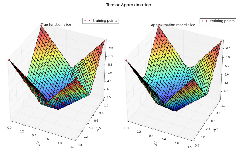
12.3.3. Tensor Approximation

This example explains the case of using the Tensor Approximation technique of GTApprox. Its advantage is the ability to provide very fast yet accurate approximation for large samples. The training sample must have specific data structure: Tensor Approximation requires gridded data to work. An example of gridded sample is the one generated bull Full Factorial technique of GTDoE which we use here (details on this technique may be found in GTDoE user manual).

The target function we will be trying to approximate is the Sobol g-function in \(R^6\):

\begin{eqnarray} &f(\vec x) = \prod_{i=1}^6 \frac{|4x_i -2| + a_i}{1+a_i}; \; \vec x \in [0, 1]^6 \nonumber \\ &\text{where } a = [4.5, 4.5, 1, 0, 1, 9]. \nonumber \end{eqnarray}

Its definition appears in the code (see data_generator()), but we will only use it in training sample generation and for comparing the GTApprox result with the true function to assess the approximation quality, so the analytical form of the target function is not available to GTApprox.

Begin with importing modules required for sample generation and approximation. Note that this example requires Matplotlib for plotting; it is recommended to use at least version 1.1 to render the plots correctly.

from da.p7core import gtdoe, gtapprox, loggers

import numpy as np
import matplotlib.pyplot as plt
import matplotlib
from mpl_toolkits.mplot3d import Axes3D

from pprint import pprint
import time
import sys
import os

Define the method to generate \(\vec x\) values of the training sample. Note we set the GTDoE/Technique option to generate full factorial as required for Tensor Approximation technique:

def full_factorial(a, b, levels, dim):
  '''
  Generate multidimensional full factorial DoE using Generic Tool for Design of Experiment.
  '''
  generator = gtdoe.Generator()
  bounds=(np.tile(a, (1, dim))[0],np.tile(b, (1, dim))[0])
  count=levels**dim
  result = generator.build_doe(bounds, count, options={'GTDoE/Technique': 'FullFactorial'})
  return result.solutions(["x"])

We also need the method to calculate Sobol g-function values for generating the \(f\) values of the training sample and for plotting:

def data_generator(points):
  '''
  Calculate Sobol g-function on given sample.
  '''
  a = [4.5, 4.5, 1, 0, 1, 9];
  values = np.ones((points.shape[0],1))[:, 0]
  for i in range(points.shape[1]):
    values = values * (np.abs(4 * points[:, i] - 2) + a[i]) / (1 + a[i])
  return values

And the one to calculate normalized RMS error for in order to analyze the obtained GTApprox model:

def rms_ptp(model, points, trueValues, dataRange):
  '''
  Calculate normalized root mean square error.
  '''
  predictedValues = model.calc(points)[:, 0]
  return np.mean((predictedValues - trueValues)**2.0)**0.5 / dataRange

The main workflow will now consist of generating the training and test samples, setting up the GTApprox builder, building the model using the generated test sample and comparing the normalized RMS error value of the model for the points of the training and test samples.

Training sample is full factorial in \(R^6\) with 10 points along each direction, so the sample size is \(10^6\) points. We use the full_factorial() and data_generator() methods to generate \(\vec x\) (trainPoints) and \(f\) (trainValues) values of the training sample, respectively:

def main():
  print('='*50)
  print('Generate training sample.')
  numberOfPointsInFactor = 10
  problemDimension = 6
  print('Generate full factorial DoE.')
  trainPoints = full_factorial(0, 1, numberOfPointsInFactor, problemDimension)
  print('Calculate function values.')
  trainValues = data_generator(trainPoints)

Test sample is simply a set of 50 000 points distributed randomly:

  print('='*50)
  print('Generate test sample.')
  numberOfTestPoints = 50000
  print('Generate random DoE.')
  testPoints = np.random.rand(numberOfTestPoints, problemDimension)
  print('Calculate function values.')
  testValues = data_generator(testPoints)

Set up the GTApprox builder. Note that since training sample size is \(10^6\) points, HDA technique will be selected by default (see the GTApprox decision tree in user manual). HDA model training for such sample sizes usually takes a few hours (compare this to the training time of TA model which the script will output to the console). To enable the Tensor Approximation technique, we set the GTApprox/EnableTensorFeature option on:

  print('='*50)
  print('Initialize and configure GTApprox builder.')
  builder = gtapprox.Builder()
  logger = loggers.StreamLogger(sys.stdout, loggers.LogLevel.DEBUG)
  print('Set logger.')
  builder.set_logger(logger)
  print('Set logging level to debug.')
  builder.options.set('GTApprox/LogLevel', 'DEBUG')
  print("By default TA technique isn't used, so we should explicitly turn this branch of decision tree on.")
  builder.options.set('GTApprox/EnableTensorFeature', 'On')

Builder is set; build the model, note the training time:

  print('='*50)
  print('Build approximation model.')
  startTime = time.time()
  model = builder.build(trainPoints, trainValues)
  finishTime = time.time()

Print model information, training time, error values for sampled points:

  print('='*50)
  print('Information about training and model:')
  print('Sample is %s points in R%s' % (trainPoints.shape[0], str(problemDimension)))
  print('Training time is %s seconds' % (finishTime - startTime))
  dataRange = np.max(testValues) - np.min(testValues)
  print('...Calculating error on training sample...')
  print('RMS/PTP error on training sample is %s' % rms_ptp(model, trainPoints, trainValues, np.max(trainValues) - np.min(trainValues)))
  print('...Calculating error on test sample...')
  print('RMS/PTP error on test sample is %s' % rms_ptp(model, testPoints, testValues, np.max(testValues) - np.min(testValues)))
  print('Model info:')
  pprint(model.info)

Note that trainValues and testValues are the true function values generated using the analytical function definition in data_generator(). Here, we compare them to model values at the same points in design space which provides a good accuracy measure.

To visualize the result, we may plot a slice of approximation against same slice of the true function. Let’s plot a slice along \(x_1\) and \(x_2\) input components, fixing other components at 0. Add plotting call at the end of main():

  print('='*50)
  print('Plot function and its approximation.')
  plot(model, trainPoints[:numberOfPointsInFactor**2, :2], trainValues[:numberOfPointsInFactor**2], problemDimension)

Plotting method (uses Matplotlib and requires at least version 1.1 to be displayed correctly):

def plot(model, trainPoints, trainValues, problemDimension):
  '''
  Plot a slice of approximation along 1st and 2nd components of X.
  It means that X3, X4, X5 and X6 are fixed at 0 and X1, X2 is varied.
  '''
  # generate points for visualizing surface
  X12 = full_factorial(0, 1, 30, 2)
  gridPointsX1 = X12[:, 0].reshape(30, 30)
  gridPointsX2 = X12[:, 1].reshape(30, 30)
  gridPoints = np.hstack([X12, np.zeros((900, problemDimension - 2))])
  gridValues = data_generator(gridPoints)
  gridValuesPrediction = model.calc(gridPoints)
  # create figure
  fig = plt.figure(figsize = (22, 10))
  fig.suptitle('Tensor Approximation', fontsize = 18)
  # make plot for function
  ax = fig.add_subplot(121, projection='3d')
  ax.set_title('True function slice')
  ax.view_init(35, -65)
  ax.scatter3D(trainPoints[:, 0], trainPoints[:, 1], trainValues, alpha = 1.0, c ='r', marker='o', linewidth = 1, s = 50)
  scatter_proxy = matplotlib.lines.Line2D((0, 0), (1, 1), marker = '.', color = 'r', linestyle = '', markersize = 10)
  reshapeSizes = [gridPointsX1.shape]
  ax.plot_surface(gridPointsX1, gridPointsX2, gridValues.reshape(reshapeSizes[0]), rstride = 1, cstride = 1, cmap = matplotlib.cm.jet,
                  linewidth = 0.1, alpha = 0.6, antialiased = False)
  ax.set_xlabel('$X_1$', fontsize ='18')
  ax.set_ylabel('$X_2$', fontsize ='18')
  ax.legend([scatter_proxy],['training points'], loc = 'best')
  # make plot for approximation
  ax2 = fig.add_subplot(122, projection='3d')
  ax2.set_title('Approximation model slice')
  ax2.view_init(35, -65)
  ax2.scatter3D(trainPoints[:, 0], trainPoints[:, 1], trainValues, alpha = 1.0, c ='r', marker='o', linewidth = 1, s = 50)
  reshapeSizes = [gridPointsX1.shape]
  ax2.plot_surface(gridPointsX1, gridPointsX2, gridValuesPrediction.reshape(reshapeSizes[0]), rstride = 1, cstride = 1, cmap = matplotlib.cm.jet,
                   linewidth = 0.1, alpha = 0.6, antialiased = False)
  ax2.set_xlabel('$X_1$', fontsize ='18')
  ax2.set_ylabel('$X_2$', fontsize ='18')
  ax2.legend([scatter_proxy],['training points'], loc = 'best')
  # save and show plots
  title = 'tensor_approximation'
  fig.savefig(title)
  print('Plots are saved to %s.png' % os.path.join(os.getcwd(), title))
  if 'SUPPRESS_SHOW_PLOTS' not in os.environ:
    plt.show()

Finally:

if __name__ == "__main__":
  main()

To run the example, open a command prompt and execute:

python -m da.p7core.examples.gtapprox.example_tensor_approx

You can also get the full code and run the example as a script: example_tensor_approx.py.

Running the example yields an image of two slices along \(x_1\) and \(x_2\) input components, one for the true function (left), the other for constructed approximation (right):

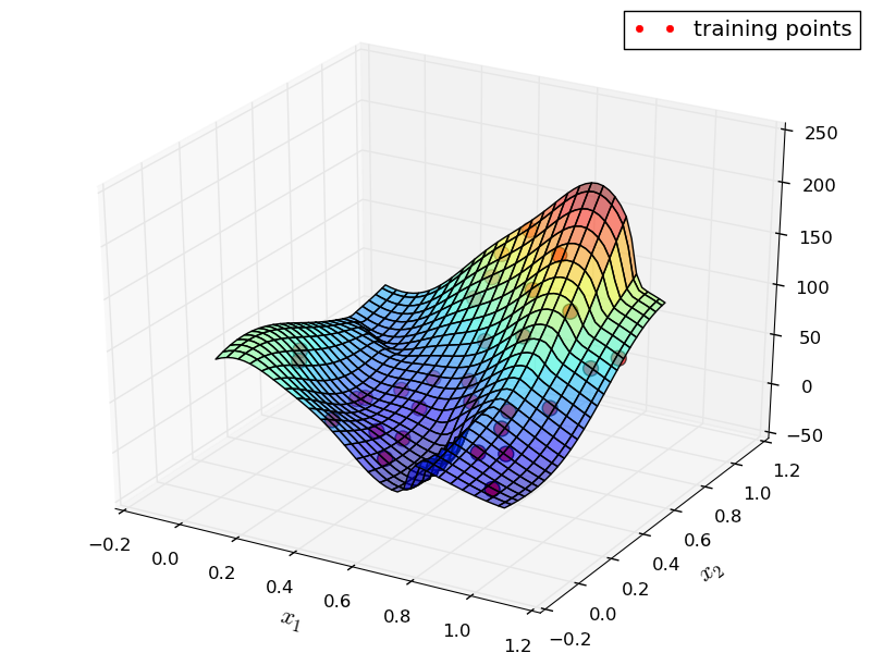
12.3.4. Mixture of Approximators Basics

The following shows how to use the Mixture of Approximators (MoA) technique of GTApprox.

Branin function

\begin{eqnarray} &f(x1,\ x2) = a \cdot (x_2 - b \cdot x_1^2 + c \cdot x_1 - d)^2 + e \cdot (1 - f) \cdot \cos(x_1) + e \nonumber \\ &a = 1,\ b = 5.1/(4\pi^2),\ c = 5/\pi,\ d = 6,\ e = 10,\ f=1/(8\pi) \nonumber \\ &-5 \leq x1 \leq 10,\ 0 \leq x2 \leq 15 \nonumber \end{eqnarray}

Start by importing required modules:

from da.p7core import gtapprox, loggers

from matplotlib import pyplot, cm, lines
from mpl_toolkits.mplot3d import Axes3D

import numpy  as np

import random

import os

12.3.4.1. Model Training

At first, define the function to be approximated:

def branin(x):
  x1 = 15 * x[:, 0] - 5
  x2 = 15 * x[:, 1]
  Y = (x2 - 5.1 / 4 / np.pi**2 * x1**2 + 5 / np.pi * x1 - 6)**2 + 10 * (1 - 1 / 8 / np.pi) * np.cos(x1) + 10
  return Y

Next step is to generate training sample to be passed to the approximator:

  dim = 2

  x_sample = np.random.rand(30, dim)
  y_sample = branin(x_sample)

Create an approximation builder (class da.p7core.gtapprox.Builder):

  builder = gtapprox.Builder()
  builder.options.set('GTApprox/Technique', 'MoA')

If you want to get some information during the training process, set a logger. We use standard da.p7core.loggers.StreamLogger. It prints logs to stdout, verbosity level is INFO.

  info_stdout_logger = loggers.StreamLogger()
  builder.set_logger(info_stdout_logger)

Now we may tune the builder (see Options Interface). Let us tune the design space decomposition algorithm specifying number of clusters and the type of covariance matrix. Number of clusters may be a single number as well as a range of possible number of clusters, in this case the best number of clusters will be selected automatically.:

  builder.options.set('GTApprox/MoACovarianceType', 'Full')
  number_of_clusters = [1, 2, 3]
  builder.options.set('GTApprox/MoANumberOfClusters', number_of_clusters)

Now, we have the training sample and the tuned approximator, so we may train it (build the surrogate model):

  model = builder.build(x_sample, y_sample)

12.3.4.2. Using the Model

Save approximation and load it from disk:

  model.save('moa_model.gta')
  loaded_model = gtapprox.Model('moa_model.gta')

Print information about the model:

  print('----------- Model -----------')
  print('SizeX: %d' % loaded_model.size_x)
  print('SizeF: %d' % loaded_model.size_f)
  print('Model has AE: %s' % loaded_model.has_ae)
  print('----------- Info -----------')
  print(str(loaded_model))

Calculate approximation at some point:

  sSize = 7
  test_xsample = [[random.uniform(0., 1.) for i in range(dim)] for j in range(sSize)]

  # calculate and display approximated values
  for x in test_xsample:
    y = loaded_model.calc(x)
    print('Model Y: %s' % y)

Calculate gradients of approximation:

  for x in test_xsample:
    dy = loaded_model.grad(x, gtapprox.GradMatrixOrder.F_MAJOR)
    print('Model gradient: %s' % dy)

The solution can be visualized using Matplotlib. Here we provide an example of how this may be done; note it requires matplotlib version at least 1.1 to be displayed correctly.

  x = np.arange(0, 1, 0.02)
  y = np.arange(0, 1, 0.02)
  x, y = np.meshgrid(x, y)
  x1 = x.reshape(x.shape[0] * x.shape[1], 1)
  x2 = y.reshape(y.shape[0] * y.shape[1], 1)
  grid_points = np.append(x1, x2, axis = 1)
  z = model.calc(grid_points)
  z = z.reshape(x.shape)

  # plot figure
  fig, ax = pyplot.subplots(subplot_kw=dict(projection='3d'))
  fig.suptitle('MoA basic', fontsize = 18)
  ax.plot_surface(x, y, z, rstride = 2, cstride = 2, cmap = cm.jet, alpha = 0.5)
  ax.scatter3D(np.array(x_sample)[:, 0], np.array(x_sample)[:, 1], y_sample, alpha = 1.0, c ='r',
               marker='o', linewidth = 1, s = 100)
  scatter_proxy = lines.Line2D((0, 0), (1, 1), marker = '.', color = 'r', linestyle = '', markersize = 10)
  ax.set_xlabel('$x_1$', fontsize ='16')
  ax.set_ylabel('$x_2$', fontsize ='16')
  ax.legend([scatter_proxy],['training points'], loc = 'best')
  ax.view_init(elev=30, azim=-60)

  fig.savefig('example_gtapprox_moa')
  if 'SUPPRESS_SHOW_PLOTS' not in os.environ:
    pyplot.show()

To run the example, open a command prompt and execute:

python -m da.p7core.examples.gtapprox.example_moa_basic

You can also get the full code and run the example as a script: example_moa_basic.py.

Running the example yields images of obtained approximation:

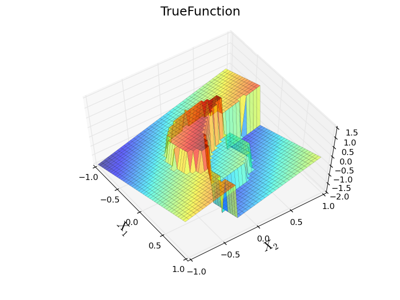
12.3.5. Mixture of Approximators Advanced

This example explains the benefits of using the Mixture of Approximators (MoA) technique. Its advantage is that it can provide higher accuracy compared to GTApprox for the functions with varying behavior across different regions of the input space — for example, the ones featuring discontinuities or discontinuous derivatives.

The target function we will be trying to approximate is given by the following formula:

\[f(x_1, x_2) = x_1 + x_2 + \boldsymbol\theta \left (x_1^2 + x_2^2 - \frac14 \right ) - 2 \boldsymbol\theta \left ( (x_1 - 0.7)^2 + (x_2 - 0.7)^2 - 1 \right).\]

Begin with importing modules required for reading samples and building approximation. Note that this example requires Matplotlib for plotting; it is recommended to use at least version 1.1 to render the plots correctly.

Import required modules:

from da.p7core import gtapprox
from da.p7core.loggers import StreamLogger

import numpy as np
from matplotlib import pyplot, cm, lines
from mpl_toolkits.mplot3d import Axes3D

import os

Define the function to be modeled:

def function(X):
  center1 = 0.5 + np.zeros((len(X), 2))
  gamma = np.ones((len(X), 2))
  Y = (np.sum(gamma * X, axis=1) + 1 * (np.sum((X - 0 * center1)**2, axis=1) <= 0.5**2) -
   2 * (np.sum((X - 0.7)**2, axis=1) <= 1**2))
  return Y

Define the method to calculate normalized RMS error in order to analyze the obtained surrogate model:

def rms(predictedValues, trueValues):
  '''
  Calculate normalized root mean square error.
  '''
  dataRange = np.max(trueValues) - np.min(trueValues)
  return np.sqrt(np.mean((predictedValues - trueValues)**2.0)) / dataRange

The main workflow will now consist of generating the training and test samples, setting up the GTApprox builder, building the models using training sample and calculating normalized RMS error of built models on test sample.

Samples were generated using uniform sampling from \([-1, 1]^2\) domain, the training sample size is 150 points. Test sample was also generated randomly from the same domain. Test sample size is 1000 points.

Generate the training sample:

  print("Generate training data")
  train_sample_size = 150
  number_of_clusters = list(range(2, 11))
  dim = 2
  x_sample = -1 + 2 * np.random.rand(train_sample_size, dim)
  y_sample = function(x_sample)

Set up the GTApprox builder and set GTApprox/Technique to 'MoA':

  print('Initialize and configure GTApprox Builder.')
  moa_builder = gtapprox.Builder()
  print('Set logger.')
  logger = StreamLogger()
  moa_builder.set_logger(logger)
  print('Set logging level to Info.')
  moa_builder.options.set('GTApprox/LogLevel', 'Info')
  print('Set approximation technique to "MoA"')
  moa_builder.options.set('GTApprox/Technique', 'MoA')

Specify approximation technique. To enable the Gaussian Process technique, we set the GTApprox/MoATechnique option to 'GP':

  print('Set approximation technique for local models to "GP"')
  moa_builder.options.set('GTApprox/MoATechnique', 'GP')

Now let us tune the design space decomposition technique. We set GTapprox/MoACovarianceType to 'Full' and specify the number of clusters as the value of the GTApprox/MoANumberOfClusters option:

  print('Set approximation technique for local models to "GP"')
  moa_builder.options.set('GTApprox/MoATechnique', 'GP')
  #[4-3]
  print('Set type of covariance matrix to "Full"')
  moa_builder.options.set('GTApprox/MoACovarianceType', 'full')
  print("Define possible number of clusters")
  number_of_clusters = np.arange(2, 11)
  moa_builder.options.set('GTApprox/MoANumberOfClusters', number_of_clusters)

Builder is set; now build the model:

  print('='*50)
  print("Building MoA model...")
  moa_model = moa_builder.build(x_sample, y_sample)

Set up GTApprox builder and construct single approximator:

  print('Initialize and configure GTApprox model for single approximation.')
  gtapprox_builder = gtapprox.Builder()
  print('Set logger.')
  gtapprox_builder.set_logger(logger)
  print('Set logging level to Info.')
  gtapprox_builder.options.set('GTApprox/LogLevel', 'Info')
  print('Set approximation technique to "GP"')
  gtapprox_builder.options.set('GTApprox/Technique', 'GP')

  print('='*50)
  print("Building single surrogate model...")
  gtapprox_model = gtapprox_builder.build(x_sample, y_sample)

Now let us compare obtained surrogate models to the real values. For this purpose load the test sample, validate the models at test points and then calculate RMS errors:

  # get data for test

  x_test_sample = np.random.rand(1000, 2) * 2 - 1
  y_test_sample = function(x_test_sample)
  print("Making prediction...")
  moa_prediction = moa_model.calc(x_test_sample)
  gtapprox_prediction = gtapprox_model.calc(x_test_sample)
  print("Calculating errors...")
  gtapprox_errors = rms(gtapprox_prediction, y_test_sample)
  moa_errors = rms(moa_prediction, y_test_sample)
  print("MoA rms error: %s" % moa_errors)
  print("GP rms error: %s" % gtapprox_errors)

Visualize the results:

  print("Plotting figures...")
  plot(x_sample, y_sample, model_name='TrueFunction')
  plot(x_sample, y_sample, moa_model, 'MoA')
  plot(x_sample, y_sample, gtapprox_model, 'GP')
  if 'SUPPRESS_SHOW_PLOTS' not in os.environ:
    pyplot.show()

Plotting methods (uses Matplotlib and requires at least version 1.1 to be displayed correctly):

def plot(x_train_sample, y_train_sample, model=None, model_name=None):
  x = np.arange(-1, 1, 0.05)
  y = np.arange(-1, 1, 0.05)
  x, y = np.meshgrid(x, y)
  x1 = x.reshape(x.shape[0] * x.shape[1], 1)
  x2 = y.reshape(y.shape[0] * y.shape[1], 1)
  grid_points = np.append(x1, x2, axis = 1)

  fig = pyplot.figure()
  fig.suptitle('MoA discontinuous function', fontsize=18)
  ax = fig.add_subplot(111, projection='3d')
  ax.set_title(model_name, fontsize=12)
  ax.view_init(azim=-35, elev=60)

  if model is None:
    z = function(grid_points)
    z = z.reshape(x.shape)
  else:
    z = model.calc(grid_points)
    z = z.reshape(x.shape)
    ax.scatter3D(x_train_sample[:, 0], x_train_sample[:, 1], y_train_sample,
                 c='r', marker='o', s=20)
    scatter_proxy = lines.Line2D((0, 0), (1, 1), marker='.', color='r',
                                 linestyle='', markersize=10)
    ax.legend([scatter_proxy],['training points'], loc='best')

  ax.plot_surface(x, y, z, rstride=1, cstride=1, cmap=cm.jet,
                  linewidth=0.1, alpha=0.6, antialiased=True)

  ax.set_xlabel('$X_1$', fontsize='18')
  ax.set_ylabel('$X_2$', fontsize='18')
  pyplot.xlim(-1, 1)
  pyplot.ylim(-1, 1)


  # save and show plots
  title = 'moa_example_discontinuous_function_' + model_name
  fig.savefig(title)

To run the example, open a command prompt and execute:

python -m da.p7core.examples.gtapprox.example_moa_discontinuous_func

You can also get the full code and run the example as a script: example_moa_discontinuous_func.py.

Running the example yields images of two surrogate models and the true function:

12.3.6. Output Variance

In many experiments it is possible to measure quality of obtained result. For example, if we can carry on experiment at the same conditions several times, then we can average results to get more precise result value and estimate uncertainty of obtained result value. GT Approx takes into account information about uncertainty of output values through the field \(outputNoiseVariance\). This example considers the case of provided estimate of output variances and compare quality of approximation of a target function with and without usage of information about output variances. Quality of approximation improves even if output variances are known only for some points. The example shows benefits of usage of output noise variance. The reason why provided output variances lead to improvement of approximation quality is that we know quality of provided function values, so we can pay more attention to points with small variance and be more careful about usage of values with big variances.

We approximate the target function below:

\[f(x) = \sin \left( \tilde{x} \right) \exp \left( -\tilde{x}^2 \right), \tilde{x} = 4.5 (x - 0.7).\]

The problem is that we can measure only noisy version of this function for points \(x \in \mathbb{X}\). Moreover, noise variance \(s^2(x)\) depends on the point location \(x\) in the following way:

\[s^2(x) = 0.001 + 0.2 x [x > 0.3],\]

where \([\cdot]\) is the indicator function, i.e. if \(x > 0.3\) then \([x > 0.3]\) equals \(1\), otherwise \([x > 0.3]\) equals \(0\). Noise is independent and Gaussian at each point, it has zero mean and specified above variance.

The example generates a training sample which models behaviour described above. Then we estimate the target function values and noise variances for each point from the training sample with multiple noisy function evaluations at each training point.

We use the following technique to estimate mean and noise variance at each training point. Suppose for a point \(x\) we have a vector of noisy function values \(\{f_j\}_{j = 1}^{N_{x}}\). Each \(f_j\) equals of sum of the target function value at this point \(f(x)\) and random noise with zero mean and variance which depends on \(x\). Then unbiased estimate of the target function value at this point has the form:

\[\overline{f}(x) = \frac{1}{N_{x}} \sum_{j = 1}^{N_{x}} f_j.\]

This value is the mean of all noisy target function values at this point. Unbiased estimate of variance of \(f_j\) for noisy function values is

\[s^2(f) = \frac{1}{N_{x} - 1} \sum_{j = 1}^{N_{x}} (f_j - \overline{f}(x))^2.\]

But we need not \(f_j\) variances estimations, but variance estimation for \(\overline{f}(x_i)\). It follows from simple math that the following unbiased estimate for \(s^2(\overline{f}(x_i))\) of \(\overline{f}(x_i)\) is:

\[\hat{s}^2(\overline{f}(x)) = \frac{1}{N_{x}} s^2(f) = \frac{1}{N_{x}} \frac{1}{(N_{x} - 1)} \sum_{j = 1}^{N_{x}} (f_j - \overline{f}(x))^2.\]

Using obtained estimate of function values and output variances we run \(GTApprox\) with and without estimates of output variances provided and compare quality of approximations for the given sample. We pay attention to both quality of approximation \(\hat{f}\) and quality of accuracy evaluation \(\hat{\sigma}^2\).

To compare two models we use the relative root-mean-squared (RRMS) error values of approximation for the test sample:

\[\rm{RRMS} = \sqrt{ \frac{\frac{1}{N_{ref}} \sum_{i = 1}^{N_{ref}} (f_i - \hat{f}_i)^2} {\frac{1}{N_{ref}} \sum_{i = 1}^{N_{ref}} (f_i - \bar{f})^2} }.\]

where \(N_{ref}\) is the test sample size, \(f_i = f(x_i)\) are function values, \(\bar{f}\) is the mean of \(f(x)\) over the test sample, \(\hat{f}_i = \hat{f}(x_i)\) are model values. RRMS error shows how accurate the model is, compared to a trivial constant approximation.

To compare accuracy evaluations quality we use correlation coefficient calculated using true errors \(|f(x) - \hat{f}(x)|\) of approximation and accuracy evaluation \(\hat{\sigma}(x)\) :

\[\rm{Corr}_{AE} = \frac{\mathrm{Cov}(|f(x) - \hat{f}(x)|, \hat{\sigma}(x))}{\sqrt{\mathrm{Cov}(|f(x) - \hat{f}(x)|, f(x) - \hat{f}(x)|), \mathrm{Cov}(\hat{\sigma}(x), \hat{\sigma}(x))}},\]

here \(\mathrm{Cov}\) is a sample covariance coefficient estimated using a sample of \(f(x), \hat{f}(x), \hat{\sigma}(x)\) values. For two vectors \(\mathbf{a} = \{a_1, \ldots, a_N \}\) and \(\mathbf{b} = \{b_1, \ldots, b_N \}\) of size \(N\) it equals:

\[\mathrm{Cov}(\mathbf{a}, \mathbf{b}) = \frac{1}{N - 1} \sum_{i = 1}^N (a_i - \bar{a}) (b_i - \bar{b}),\]

where \(\bar{a}\) is the mean of \(\mathbf{a}\), \(\bar{b}\) is the mean of \(\mathbf{b}\).

Again, to calculate covariances for actual errors and accuracy evaluations we use the test sample.

To make clear the difference between two models we plot approximations and corresponding accuracy evaluations.

Note that this example requires Matplotlib for plotting. Version 1.1 or later is recommended to display the plots correctly.

Script starts with import of modules:

import os

import matplotlib.pyplot as plt
import numpy as np

from da.p7core import gtapprox, gtdoe

The target function has the form:

def target_function(x, shift=0.7, scale=4.5):
  """
  Target function with 1D input.

  Args:
    x: 1D point or a NumPy array.
    shift, scale: the target function optional parameters

  Returns:
    Single function value or an array of values. Array shape is the same
    as input shape.
  """
  x_tilde = (x - shift) * scale
  result = np.sin(x_tilde) * np.exp(-x_tilde ** 2)
  return result

Training sample generation function uses GT DoE \(LHS\) (Latin Hyper Cube) technique. The training points generation is presented below:

  generator = gtdoe.Generator()

  # set DoE options
  options = {"GTDoE/Technique": "LHS",
             "GTDoE/Deterministic": "yes",
             "GTDoE/Seed" : 200}
  generator.options.set(options)

  # generate points using GT DoE
  points = generator.generate(bounds=bounds,
                              count=points_number).points.reshape(-1, 1)

To estimate noise variance at each point we need to calculate noisy function at this point multiple times, so noisy function output consists of specified number of noisy true function values at specified point. We generate noisy target function values with the code:

  values = []
  for point in points:
    # get noise variance for the point
    point_noise_variance = 10e-4 + 0.2 * point * (point > 0.3)
    # generate noised function values
    values.append(target_function(point) +
                  point_noise_variance ** 0.5 *
                  np.random.randn(point_evaluation_number, 1))

For a sample generated in such a way we can estimate both mean value and noise variance at each point from the training sample.

def estimate_noise_variances(training_values):
  """
  Estimate noise variances and mean at each input point.
  Mean estimation is straightforward.
  We use unbiased variance estimation with assumption about zero mean for noise values.
  We begin with variance estimation for provided values at each point.
  Then we obtain variance estimation for mean of provided values at each point.

  Args:
    training_values: training outputs, NumPy array.

  Returns:
    NumPy array of function values estimation and corresponding noise variances estimation at each point.
  """

  training_mean_values = []
  training_output_variance_values = []
  for point_values in training_values:
    training_mean_values.append(np.mean(point_values))
    training_value_variance_estimation = (np.sum((point_values - np.mean(point_values)) ** 2) /
                                          (point_values.shape[0] - 1))
    training_mean_value_variance_estimation = (training_value_variance_estimation /
                                               point_values.shape[0])
    training_output_variance_values.append(training_mean_value_variance_estimation)
  return training_mean_values, training_output_variance_values

For demonstration purpose we replace some output variances values with NaNs using the function below

def mix_in_nans(values, nan_points_number):
  """
  Replace values in random points with NaNs
  Using this script we emulate unavailability
  of provided output variances for some training points

  Args:
    values: initial input sample
    nan_points_number: number of points to replace with NaNs

  Return values with nans inserted
  """
  points_number = np.shape(values)[0]

  permuted_indexes = np.random.permutation(list(range(points_number)))

  nan_indexes = permuted_indexes[:nan_points_number]
  for index in nan_indexes:
    values[index] = np.nan
  return values

Now one can use the results below to get a training sample which one can pass to GT Approx. We run GT Approx in two modes: with and without usage of estimated output variances.

def build_models(training_points, training_values, training_output_variance_values):
  """
  Build models for the given training sample with and without output variances provided

  Args:
    training_points: training inputs, NumPy array.
    training_values: training outputs, NumPy array.
    training_output_variance_values: training output variances, NumPy array.

  Returns:
    Models obtained with and without usage of output variances
  """
  builder = gtapprox.Builder()
  builder.options.set({"GTApprox/Technique" : "GP",
                       "GTApprox/AccuracyEvaluation" : "on"})
  model = builder.build(training_points, training_values)
  model_with_output_variances = builder.build(training_points, training_values, outputNoiseVariance=training_output_variance_values)
  return model, model_with_output_variances

We compare RRMS for approximations and correlations for accuracy evaluations.

def validate_models(models, test_sample):
  """
  Validate constructed models using a test sample.
  We calculate RRMS errors and correlation between the true residuals and accuracy evaluation

  Args:
    models: two models constructed with GT approximation.
    test_sample: test points and corresponding test values.
  """
  model, model_with_output_variances = models
  test_points, test_values = test_sample

  print("Validating of model without usage of output variances")
  validation_result_model = model.validate(*test_sample)
  print("Validating of model with usage of output variances")
  validation_result_model_with_output_variances = model_with_output_variances.validate(*test_sample)
  print("Get approximation and accuracy evaluation for model without usage of output variances")
  model_values = model.calc(test_points)
  model_ae = model.calc_ae(test_points)
  print("Get approximation and accuracy evaluation for model with usage of output variances")
  model_with_output_variances_values = model_with_output_variances.calc(test_points)
  model_with_output_variances_ae = model_with_output_variances.calc_ae(test_points)
  ae_correlation = np.corrcoef(np.abs(model_values - test_values),
                                  model_ae, rowvar=0)[0, 1]
  ae_with_output_variances_correlation = np.corrcoef(np.abs(model_with_output_variances_values - test_values),
                                              model_with_output_variances_ae, rowvar=0)[0, 1]

  print("\tModel without usage of output variances RRMS: %s" % validation_result_model["RRMS"][0])
  print("\tModel with usage of output variances RRMS: %s" % validation_result_model_with_output_variances["RRMS"][0])
  print("\tAE for model without usage of output variances correlation: %s" % ae_correlation)
  print("\tAE for model with usage of output variances correlation: %s" % ae_with_output_variances_correlation)

We get the following output:

Model without usage of output variances RRMS: 0.365073606139
Model with usage of output variances RRMS: 0.212741595938
AE for model without usage of output variances correlation: -0.198709325888
AE for model with usage of output variances correlation: 0.586275220152
Models validated.

In this case usage of output variances improves quality of both approximation and accuracy evaluation: RRMS for model with usage of output variances is smaller and correlation for accuracy evaluation if output variances are used is bigger.

After validation, the script displays two figures: obtained approximations and accuracy evaluation vs true function and true errors correspondingly:

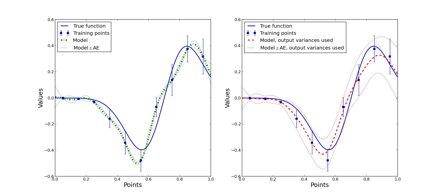
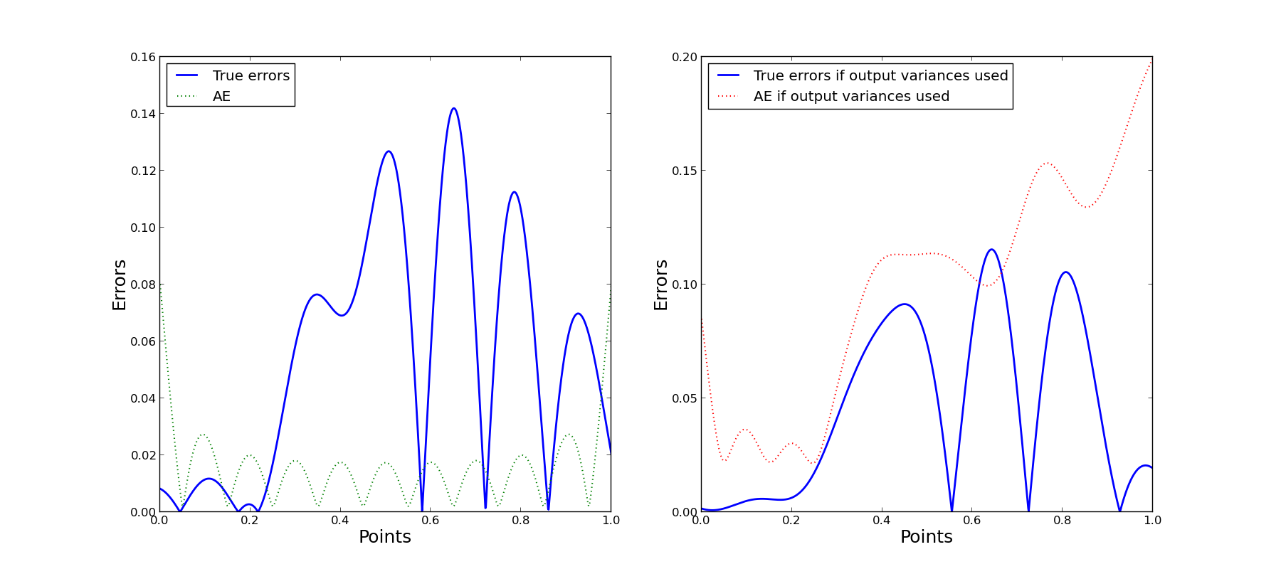
From the above figures it follows that in case we use estimates of output variances the approximation quality is better. Accuracy evaluation is also more adequate if output variances are used. Note, that accuracy evaluation isn’t intended for prediction of the actual error, but provides uncertainty estimation for the corresponding approximation at the point and contains information about a local function behavior.

Note that for some points AE is significantly bigger than zero, but actual error value is zero. The reason is that for this one-dimensional function zero errors outside the training sample appears due to accident intersection of approximation and the true function. It is natural that we can’t predict such a peculiarity and corresponding AE value is significantly bigger than zero.

To run the example, open a command prompt and execute:

python -m da.p7core.examples.gtapprox.example_output_variances

You can also get the full code and run the example as a script: example_output_variances.py.

12.3.7. Additive Covariance Function

This toy example demonstrates usage of different covariance functions for GP technique. Also it demonstrates how one can improve approximation of a true function by incorporating a special knowledge about the data structure. We paid special attention to additive covariance function as it can handle specific true function structure, moreover one can often benefit from usage of this covariance function even if one can say nothing for sure about the true function especially if data input dimension \(d\) is huge.

We approximate the artificial target function below with input dimension \(d = 2\):

\[f(x) = \sum_{i = 1}^{d} \sin \left(10 x_i \right).\]

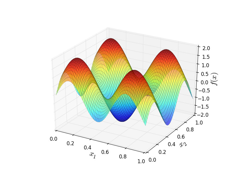
As one can see this function has additive structure so the additive covariance function suits perfectly for it.

The example generates a training sample of size \(15\). Points from the training sample are generated from the uniform distribution on the unit cube \([0, 1]^2\). Then we construct three different models with three different sets of options. Options for the first model construction is default. For the second model we use Mahalanobis covariance function instead of weighted \(l_p\) covariance function used by default. For the third model we use Additive covariance function.

Then we compare obtained models in terms of RRMS error and visually.

Script starts with import of modules.

import os

import numpy as np
import matplotlib.pyplot as plt
from matplotlib import cm
from mpl_toolkits.mplot3d import Axes3D

from da.p7core import gtapprox

The target function has the form:

def target_function(x):
  """
  Example target function with additive structure.

  Args:
    x: 2D NumPy array.

  Returns:
    An array of the target function values.
    Number of elements in output array coincides with number of input points.
  """
  result = np.sum(np.sin(10 * x), axis=1)
  return result

Training sample consists of points uniformly space over the domain \([0, 1]^2\).

  print("=" * 50)
  print("Training sample generation...")
  training_points = np.random.rand(15, 2)
  training_values = target_function(training_points)
  training_sample = (training_points, training_values)

We pass the generated training sample to GTApprox with different options: default options, Mahalanobis covariance function and Additive covariance function. To set covariance function we modify value of GTApprox/GPType option.

def construct_models(training_points, training_values):
  """
  Construct required surrogate models with pSeven Core GT Approx.

  Args:
    training_points: training points, 2D NumPy array.
    training_values: training values, NumPy array.

  Returns:
    three constructed surrogate model
  """
  builder = gtapprox.Builder()
  print("Construct surrogate model with default options...")
  default_model = builder.build(training_points, training_values, {})

  print("Construct surrogate model with Mahalanobis covariance function...")
  mahalanobis_covariance_function_model = builder.build(training_points, training_values,
                                                        {"GTApprox/GPType" : "Mahalanobis"})

  print("Construct surrogate model with Additive covariance function...")
  additive_covariance_function_model = builder.build(training_points, training_values,
                                                     {"GTApprox/GPType" : "Additive"})
  return (default_model,
          mahalanobis_covariance_function_model,
          additive_covariance_function_model)

We compare RRMS errors for a test sample. Smaller values of errors are better as we want to construct a model that resembles the target function as accurate as possible. We run the following code:

def validate_models(models):
  """
  Calculate RRMS errors of constructed surrogate models for a test sample
  and correlations between true values and outputs of the constructed surrogate models.

  Args:
    models: a tuple which contains surrogate models constructed with GT Approx .
  """
  (default_model,
   mahalanobis_covariance_function_model,
   additive_covariance_function_model) = models

  print("Test sample generation...")
  test_points = np.random.rand(1000, 2)
  test_values = target_function(test_points)
  test_sample = (test_points, test_values)

  print("Test sample validation result...")
  print("RRMS error for GTApprox model with default options: %s" %
        (default_model.validate(*test_sample)["RRMS"][0]))
  print("RRMS error for GTApprox model with Mahalanobis covariance function: %s" %
        (mahalanobis_covariance_function_model.validate(*test_sample)["RRMS"][0]))
  print("RRMS error for GTApprox model with Additive covariance function: %s" %
        (additive_covariance_function_model.validate(*test_sample)["RRMS"][0]))

And we get the following output:

Test sample validation result...
  RRMS error for GTApprox model with default options: 0.696878291677
  RRMS error for GTApprox model with Mahalanobis covariance function: 0.675345818614
  RRMS error for GTApprox model with Additive covariance function: 0.0440210069708

As one can see, we obtain the best result in case we use Additive covariance function.

After validation, the script displays four subfigures: the target function and obtained approximations plots. We also display locations of the training points with black circles. To generate each subplot we use the following code:

  def plot_contour_figure(test_points, test_values, training_points, title):
    """
    Plot a single contourf subplot for specified values.

    Args:
      test_points: 2d array of test tensor points to plot.
      test_values: vector array of test tensor values to plot.
      training_points: design of experiments for the training sample.
    """
    ax = figure_handle.add_subplot(2, 2, index + 1)
    ax.set_xlim([0, 1])
    ax.set_ylim([0, 1])

    # Set text for subplot
    ax.set_title(title, fontsize=12)
    ax.set_xlabel("$x_1$", fontsize=16)
    ax.set_ylabel("$x_2$", fontsize=16)

    # Contour plot for the given data
    ax.contourf(test_points[:, 0].reshape(mesh_size[0], mesh_size[1]),
                test_points[:, 1].reshape(mesh_size[0], mesh_size[1]),
                test_values.reshape(mesh_size[0], mesh_size[1]),
                levels=contour_levels)

    # Add training sample scatter
    ax.scatter(training_points[:, 0], training_points[:, 1],
               s=60, vmin=0, vmax=1, linewidth=1.5,
               c=(training_values - min_value) / (max_value - min_value))

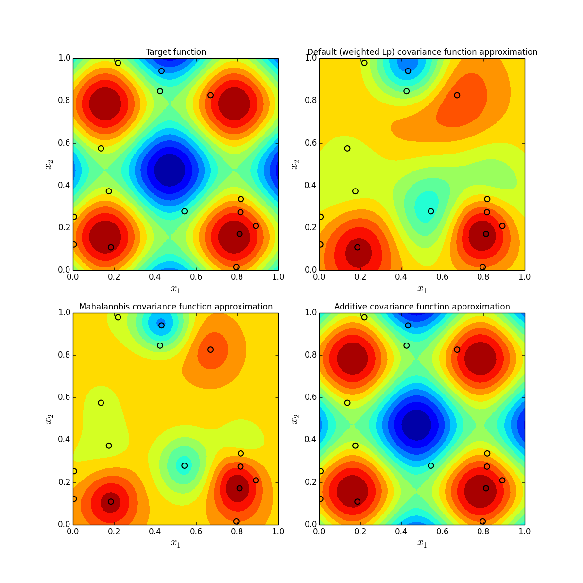
One can see that in case we use Additive covariance function the approximation is almost perfect even for a training sample of small size. For other covariance functions we need more points to obtain an approximation of a comparable quality.

Note, that the additive covariance function is also useful in the case of huge input dimension \(d\).

To run the example, open a command prompt and execute:

python -m da.p7core.examples.gtapprox.example_additive_gp

You can also get the full code and run the example as a script: example_additive_gp.py.

12.3.8. Training with Limited Memory

This example illustrates an approach that allows to train a surrogate model with a sample that is too big to be handled at once (can cause memory overflow when training). The example utilizes the GTApprox/MaxExpectedMemory option and performs simple partitioning of the training sample to “fit” the model builder in the available memory.

Note

This example can run long, up to several hours on low performance systems.

Note that GTApprox/MaxExpectedMemory is supported only by the GBRT technique. It’s important to note that this option controls only amount of memory spent to model building process, and it does not take into account memory spent due to various memory management mechanisms in operational system or say data caching in python. So sometimes set limit can be violated.

When memory used by build() exceeds specified limit building stops and last correct state of the model is returned. Special field /GTApprox/MemoryOverflowDetected is added to model.info['ModelInfo']['Builder']['Details'], indicating that memory limitation was violated. After the event occurred user may split sample in several smaller parts and update current model state with each part sequentially.

Note that if the sample is so big that model training (or updating) process didn’t even manage to start OutOfMemoryError exception is raised and no model object is returned.

First of all we do all necessary imports.

import sys
import traceback
import numpy as np

from da.p7core import gtapprox
from da.p7core.loggers import StreamLogger

We also define simple function we would generate training sample with.

def function(X):
  Y = np.sum(X**2, axis=1) + 1
  return Y[:, np.newaxis]

This code generates quite big sample:

  print("Generate training data")
  train_sample_size = 1000000
  dim = 128
  x_sample = -1 + 2 * np.random.rand(train_sample_size, dim)
  y_sample = function(x_sample)

We set the limit we put on used memory (note that minimum size that can be set is 1 Gb, setting 0 means that limit on memory usage is disabled). In this example the limit is set to be 10% of all free system memory, but no less than 1 Gb. The example uses psutil if available to estimate the amount of free memory.

  try:
    import psutil
    all_free_memory = psutil.virtual_memory().available/1024./1024./1024. # in Gbs
    print('%s Gb is free.' % all_free_memory)
    # we allow builder to use up to 10% of all memory
    max_allowed_memory = np.max((round(0.1 * all_free_memory), 1))
  except:
    # if psutil is not installed or other error occurred we just set limit to 1 Gb
    max_allowed_memory = 1

  print('%s Gb may be used to construct model.' % max_allowed_memory)

After that the model building process with memory limit is started.

  model = build_with_memory_control(x_sample, y_sample, max_allowed_memory=max_allowed_memory)
  model.save('model.gtapprox')

Here is the code of build_with_memory_control function that handles the building.

def build_with_memory_control(x, y, max_allowed_memory, sample_split_coefficient=1.6):

  print('\nModel building process started...\n')

  number_of_parts = 1  # at first no splitting is done
  unprocessed_offset = 0  # current offset of processed points
  number_of_points = x.shape[0]
  model = None  # no initial model is initialized

  while unprocessed_offset < number_of_points:  # training continues until all data is processed
    # this line gets number of points that would be used in the next training attempt
    number_to_process = round((number_of_points - unprocessed_offset)/float(number_of_parts))

    processing_end_offset = int(np.min((unprocessed_offset + number_to_process, number_of_points)))

    offsets = (unprocessed_offset, processing_end_offset)

    # this function runs the building attempt
    model, status = build_attempt(x, y, offsets, initial_model=model, max_allowed_memory=max_allowed_memory)

    # here function processes building attempt outcome
    if status:
      # building succeeded
      number_of_parts -= 1
      unprocessed_offset = processing_end_offset
      print('')
      print('Updated model for %dpoints.' % int(number_to_process))
      print('%d unprocessed points remain.' % int((number_of_points - unprocessed_offset)))
      print('Unprocessed data is split in %d parts now.' % int(number_of_parts))
      print('')
    else:
      # building failed, we split data more
      number_of_parts = round(sample_split_coefficient * number_of_parts)
      print('')
      print('Failed to build model for %d points.' % int(number_to_process))
      print('%d unprocessed points remain.' % int((number_of_points - unprocessed_offset)))
      print('Unprocessed data is split in %d parts now.' % int(number_of_parts))
      print('')

  return model

Function tries to build the model using all the sample at first. If building failed it splits the sample using given \(sample\_split\_coefficient\) argument value to define the splits. If successful it updates the model with next available split.

Each building attempt is done in build_attempt function, which checks if model build was successful and if there is a model that can be returned for further update.

def build_attempt(x, y, offsets, initial_model=None, max_allowed_memory=0):

  if len(y.shape) == 1:
      y = y[:, np.newaxis]

  try:
    # function tries to build (or if initial_model is not None to update) the model
    builder = gtapprox.Builder()
    builder.set_logger(StreamLogger())

    model = builder.build(x[offsets[0]:offsets[1], :], y[offsets[0]:offsets[1], :],
                                     options={'GTApprox/Technique': 'GBRT',
                                              'GTApprox/MaxExpectedMemory': max_allowed_memory})

    # if no exception was raised function checks if memory overflow occurred
    if ('/GTApprox/MemoryOverflowDetected' in model.info['ModelInfo']['Builder']['Details'])\
      and (model.info['ModelInfo']['Builder']['Details']['/GTApprox/MemoryOverflowDetected']):
      status = False
    else:
      status = True

    # note that even if memory overflow occurred model could still be updated to some extent
    # so in such case we always return modified model object

  except Exception:
    # here function processes the exception if any occurred
    traceback.print_exception(*sys.exc_info())
    model = initial_model # if exception occurred initial_model returns unchanged
    status = False

  return model, status  # status True means that build was successful

You can also get the full code and run the example as a script: example_memory_control.py.

12.3.9. Checking Model Domain

This example illustrates one of the possible approaches to checking whether certain input data belogs to the model’s validity domain.

Exact definition of a validity domain can be very different as it depends on data, problem statement, model type and so on. In this example the validity domain means a region where you can trust model predictions.

When checking if you should trust model predictions in given point, first of all you should check whether you are operating is in interpolation or extrapolation mode (as models often are unreliable outside the training data). The easiest check you can do is to look if the considered point lies inside or outside the boundaries of the hypercube that encloses the training sample. It allows to quickly find points that are far away from the training sample and in which you should not trust model predictions.

The other approach you can use for the points that are not far away from the training sample is to construct a classifier model that tells in which points the model gives accurate enough predictions. To do so we set the acceptable level of prediction accuracy, limiting the relative error to 10%. After that we train a model that tells whether the relative error in a new point is estimated to be less than 10%.

The example demonstrates implementation of both checks. The target function it uses to generate data and test the models is:

\[f(x_1, x_2) = \bigl|2 + \sin(4 x_1 + 4 x_2) + 0.5 \varepsilon\bigr|,\]

where \(\varepsilon\) is the standard normal noise.

The example consists of the following parts:

1. Generate the training and test samples.
2. Train an approximation model. To obtain a training sample for the classifier (containing model error estimates), we also enable internal validation when training the model.
3. Check if test sample points lie inside the hypercube containing the training data.
4. Train an additional classifier model that predicts whether the main model is accurate enough in a considered point.
5. To evaluate classifier accuracy we draw the ROC-curve on test data.

Begin with importing modules. Note that this example requires Matplotlib for plotting.

import os
import matplotlib.pyplot as plt
import numpy as np

from da.p7core import gtapprox, loggers

The target function is:

def true_function(points, noise_variance=0.005):
  """ A simple noised function we will use to study approximation validity domain.
  """
  values = 2 + np.sin(np.sum(4 * points, axis=1, keepdims=True))
  values = values + noise_variance ** 0.5 * np.random.randn(np.shape(values)[0],
                                                            np.shape(values)[1])
  values = np.abs(values)
  return values

First of all the user has to define what accuracy (relative error) is acceptable.

  """
  Here we set relative error bound on acceptable accuracy.
  """
  relative_error_bound = 0.1

The training and test samples consist of points uniformly spaced over the \([0, 1]^2\) domain.

  """
  Here we generate train and test data.
  """
  training_points, training_values = get_data(300)
  test_points, test_values = get_data(10000)

Generate samples:

def get_data(sample_size=200, input_dimension=2):
  """ Get data randomly distributed in a unit hypercube
  """
  points = np.random.rand(sample_size, input_dimension)
  values = true_function(points)

  return points, values

After that we use the training sample to build the approximation model. We enable Internal Validation to get information on model prediction accuracy via option GTApprox/InternalValidation. Note that we use GTApprox/IVSavePredictions to save internal validation predictions (we will use them to train the classifier at the next step). After that all data is available in the model’s iv_info.

  """
  Here we construct approximation model.

  Note that we turn on internal validation to get the information on model accuracy.
  And we save internal validation predictions and get them from model to use them
  for constructing accuracy model.
  """
  print("Building initial surrogate model...\n")
  builder = gtapprox.Builder()
  builder.set_logger(loggers.StreamLogger())
  model = builder.build(training_points, training_values,
                        options={'GTApprox/Technique': 'GP',
                                 'GTApprox/InternalValidation': 'on',
                                 'GTApprox/IVSavePredictions': 'on',
                                 'GTApprox/IVSubsetCount': 10,
                                 'GTApprox/IVTrainingCount': 10,
                                })

  print("Done.\n")

  internal_validation_inputs = model.iv_info['Dataset']['Validation Input']
  internal_validation_outputs = model.iv_info['Dataset']['Validation Output']
  internal_validation_predictions = model.iv_info['Dataset']['Predicted Output']

We use this internal validation data to construct the classifier that tries to determine if the model is accurate in a given new point.

  """
  Here we construct classifier that predicts model accuracy
  """
  print("Constructing classifier that tells if prediction in point would be accurate...")
  validity_classifier = construct_classifier(internal_validation_inputs,
                                             internal_validation_outputs,
                                             internal_validation_predictions,
                                             relative_error_bound)
  print("Done.\n")

See the code of the function:

def construct_classifier(points, values, predictions, relative_error_bound=0.1):
  """ Construct classifier that returns probability that model gives good prediction
  in considered point i.e. relative error is smaller than relative_error_bound
  """
  relative_errors = np.abs(values - predictions) / (np.abs(values) + 1e-9)
  # 1e-9 is added here to ensure that no problem occur in cases true value = 0

  # Construct classifier
  builder = gtapprox.Builder()
  builder.set_logger(loggers.StreamLogger())
  validity_classifier = builder.build(points, relative_errors < relative_error_bound,
                                      options={'gtapprox/technique': 'gbrt',
                                               '/GTApprox/GBRTObjective': 'binary:logistic'})

  return validity_classifier

After that we check if the test sample lies inside the same region as the training sample and find points that are located outside. Good rule generally is not to predict anything in the points lying outside.

  """
  Here we take data on training sample properties and check if test set points lie inside
  """

  print("Checking if points lie inside input domain...\n")
  points_lie_inside = np.ones(test_values.shape, dtype=np.bool_)

  input_sample_stats = model.details['Training Dataset']['Sample Statistics']['Input']

  for dimension in range(len(input_sample_stats['Count'])):
    check_dimension = (input_sample_stats['Min'][dimension] <=
                       test_points[:, dimension:dimension+1])
    check_dimension *= (test_points[:, dimension:dimension+1] <=
                        input_sample_stats['Max'][dimension])
    points_lie_inside = np.logical_and(points_lie_inside, check_dimension)
  print("Result:")
  print("%s points lie inside train sample area" % np.sum(points_lie_inside == True))
  print("%s points lie outside train sample area\n" % np.sum(points_lie_inside == False))

As a second action we use our classifier model on test data to see where model predictions are good. We compute classifier predictions on test and prepare test data labels:

  """
  Prepare test data predictions and true labels.
  """
  print("Using classifier to check accuracy in points...\n")
  sim_values = model.calc(test_points)
  valid_model_probability = validity_classifier.calc(test_points)

  sim_values_validity = np.abs((test_values - sim_values) / test_values)

And finally we draw ROC curve to check accuracy metrics of classifier.

  """
  Draw ROC curve.
  """
  plot_roc_curve(sim_values_validity < relative_error_bound, valid_model_probability)

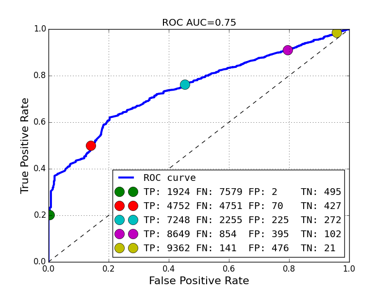
We need some custom code to draw such ROC curve:

def calculate_auc(x_axis_values, y_axis_values):
  """ Get area under curve
  x axis values are sorted in ascending order
  """
  return np.trapz(y_axis_values, x_axis_values)
#[4]

#[5]
def get_fp_tp_curve(y_true, y_score):
  """ Get False Positive and True Positive values for various thresholds
  """
  # Ravel data
  y_true = y_true.ravel()
  y_score = y_score.ravel()

  # Sort scores and corresponding truth values
  descending_sort_indices = np.argsort(y_score)[::-1]
  y_score = y_score[descending_sort_indices]
  y_true = y_true[descending_sort_indices]

  # Use only distinct scores
  distinct_value_indices = np.where(-np.diff(y_score) > 1e-7)[0]
  threshold_indexes = np.r_[distinct_value_indices, len(y_true) - 1]

  # Get true positive and false positive number
  true_positive_number = (0. + y_true).cumsum()[threshold_indexes]
  false_positive_number = (1. - y_true).cumsum()[threshold_indexes]

  return false_positive_number, true_positive_number
#[5]

#[6]
def roc_curve(y_true, y_score):
  """ Get True Positive Rates and False Positive Rates for ROC curve construction
  """
  positive_number = np.sum(y_true)
  negative_number = np.sum(y_true == 0)

  false_positive_number, true_positive_number = get_fp_tp_curve(y_true, y_score)

  # add first line
  if false_positive_number[0] != 0:
    true_positive_number = np.r_[0, true_positive_number]
    false_positive_number = np.r_[0, false_positive_number]

  if negative_number > 0:
    false_positive_ratio = false_positive_number / negative_number
  else:
    false_positive_ratio = np.nan * false_positive_number

  if positive_number > 0:
    true_positive_ratio = true_positive_number / positive_number
  else:
    true_positive_ratio = np.nan * true_positive_number

  return false_positive_ratio, true_positive_ratio
#[6]

#[7]
def get_roc_curve(test_values, test_sim_probabilities):
  """ Get data for ROC curve
  """
  first_axis_rate, second_axis_rate = roc_curve(test_values, test_sim_probabilities)
  auc_value = calculate_auc(first_axis_rate, second_axis_rate)
  return first_axis_rate, second_axis_rate, auc_value
#[7]

#[8]
def get_confusion_matrix_label(negative_number, positive_number, first_quantile, second_quantile, max_len):
  false_positive = int(negative_number * first_quantile)
  true_negative = negative_number - false_positive
  true_positive = int(positive_number * second_quantile)
  false_negative = positive_number - true_positive

  false_positive_string = str(false_positive)
  true_negative_string = str(true_negative)
  true_positive_string = str(true_positive)
  false_negative_string = str(false_negative)
  confusion_matrix_strings = [true_positive_string, false_negative_string,
                              false_positive_string, true_negative_string]

  confusion_matrix_strings = [x + ' ' * (max_len - len(x)) for x in confusion_matrix_strings]
  confusion_matrix_names = ['TP: ', 'FN: ', 'FP: ', 'TN: ']
  return ''.join(z + t for z, t in zip(confusion_matrix_names, confusion_matrix_strings))
#[8]

#[9]
def plot_roc_curve(test_values, test_sim_probabilities, quantile_list=[5, 25, 50, 75, 95]):
  """
    Plot Receiver operating characteristic (ROC) performance curve
    Inputs:
      test_values - numpy array of true values, 0 or 1
      test_sim_probabilities - numpy array of simulated probabilities with values inside the interval [0, 1]
      quantile_list - list of quantiles for which we display confusion matrices
    Outputs:
      auc_value - AUC value for classifier
      first_axis_rate - value for the first axis
      second_axis_rate - value for the second axis
  """
  # Get data for ROC curve
  first_axis_rate, second_axis_rate, auc_value = get_roc_curve(test_values, test_sim_probabilities)

  plt.figure()

  # Plot bisector of quadrant
  plt.plot([0, 1], [0, 1], "k--")

  # Plot rates
  plt.plot(first_axis_rate, second_axis_rate, label="ROC curve", linewidth=3)

  # Plot quantile points
  sample_size = len(test_values)
  positive_number = int(np.sum(test_values))
  negative_number = int(sample_size - np.sum(test_values))
  max_len = len(str(int(sample_size)))
  for quantile in quantile_list:
    first_quantile = np.percentile(first_axis_rate, quantile)
    second_quantile = np.percentile(second_axis_rate, quantile)

    label = get_confusion_matrix_label(negative_number, positive_number, first_quantile, second_quantile, max_len)
    plt.plot(first_quantile, second_quantile, 'o', label=label, markersize=15)

  # Set correct axis
  plt.axis([0.0, 1.0, 0.0, 1.0001])
  plt.grid(True)

  # Plot legend and labels
  plt.xlabel("False Positive Rate", fontsize=16)
  plt.ylabel("True Positive Rate", fontsize=16)
  plt.legend(loc="lower right", prop={"family" : "monospace"})
  plt.title("ROC AUC=%0.2f" % (auc_value))

  # Save file
  file_name = "roc_curve.png"
  plt.savefig(file_name)
  if 'SUPPRESS_SHOW_PLOTS' not in os.environ:
    plt.show()

  return first_axis_rate, second_axis_rate, auc_value
#[9]

To run the example, open a command prompt and execute:

python -m da.p7core.examples.gtapprox.example_get_validity_domain

You can also get the full code and run the example as a script: example_get_validity_domain.py.

12.3.10. SHapley Additive exPlanations

This example shows using gtapprox.Model.shap_value() to get SHAP values from a model. It is available as an IPython notebook: example_shap.ipynb.